This twenty-second article, which is part of the series on Linux device drivers, lays out a bare bone file system module.
With the formatting of the pen drive, the file system is all set in the hardware space. Now, it is the turn to decode that using a corresponding file system module in the kernel space, and accordingly provide the user space file system interface, for it to be browsed like any other file systems.
The 5 sets of System Calls
Unlike character or block drivers, the file system drivers involve not just one structure of function pointers, but instead 5 structures of function pointers, for the various interfaces, provided by a file system. These are:
- struct file_system_type – contains functions to operate on the super block
- struct super_operations – contains functions to operate on the inodes
- struct inode_operations – contains functions to operate on the directory entries
- struct file_operations – contains functions to operate on the file data (through page cache)
- struct address_space_operations – contains page cache operations for the file data
With these, there were many new terms for Pugs. He referred the following glossary to understand the various terms used above and later in the file system module development:
- Page cache or Buffer cache: Pool of RAM buffers, each of page size (typically 4096 bytes). These buffers are used as the cache for the file data read from the underlying hardware, thus increasing the performance of file operations
- Inode: Structure containing the meta data / information of a file, like permissions, owner, etc. Though file name is a meta data of a file, for better space utilization, in typical Linux file systems, it is not kept in inode, instead in something called directory entries. Collection of inodes, is called an inode table
- Directory entry: Structure containing the name and inode number of a file or directory. In typical Linux based file systems, a collection of directory entries for the immediate files and directories of say directory D, is stored in the data blocks of the directory D
- Super block: Structure containing the information about the various data structures of the file systems, like the inode tables, … Basically the meta meta data, i.e. meta data for the meta data
- Virtual File System (VFS): Conceptual file system layer interfacing the kernel space to user space in an abstract manner, showing “everything” as a file, and translating their operations from user to the appropriate entity in the kernel space
Each one of the above five structures contains a list of function pointers, which needs to be populated depending on what all features are there or to be supported in the file system (module). For example, struct file_system_type may contain system calls for mounting and unmounting a file system, basically operating on its super block; struct super_operations may contain inode read/write system calls; struct inode_operations may contain function to lookup directory entries; struct file_operations may generically operate on the page cached file data, which may in turn invoke page cache operations, defined in the struct address_space_operations. For these various operations, most of these functions will then interface with the corresponding underlying block device driver to ultimately operate with the formatted file system in the hardware space.
To start with Pugs laid out the complete framework of his real SFS module, but with minimal functionality, good enough to compile, load, and not crash the kernel. He populated only the first of these five structures – the struct file_system_type; and left all the others empty. Here’s the exact code of the structure definitions:
#include <linux/fs.h> /* For system calls, structures, ... */

static struct file_system_type sfs;
static struct super_operations sfs_sops;
static struct inode_operations sfs_iops;
static struct file_operations sfs_fops;
static struct address_space_operations sfs_aops;
#include <linux/version.h> /* For LINUX_VERSION_CODE & KERNEL_VERSION */

static struct file_system_type sfs =
{
	name: "sfs", /* Name of our file system */
#if (LINUX_VERSION_CODE < KERNEL_VERSION(2,6,38))
	get_sb:  sfs_get_sb,
#else
	mount:  sfs_mount,
#endif
	kill_sb: kill_block_super,
	owner: THIS_MODULE
};
Note that before Linux kernel version 2.6.38, the mount function pointer was referred as get_sb, and also, it used to have slightly different parameters. And hence, the above #if for it to be compatible at least across 2.6.3x and possibly with 3.x kernel versions – no guarantee for others. Accordingly, the corresponding functions sfs_get_sb() and sfs_mount(), are also #if’d, as follows:
#include <linux/kernel.h> /* For printk, ... */

if (LINUX_VERSION_CODE < KERNEL_VERSION(2,6,38))
static int sfs_get_sb(struct file_system_type *fs_type, int flags,
			const char *devname, void *data, struct vfsmount *vm)
{
	printk(KERN_INFO "sfs: devname = %s\n", devname);

	/* sfs_fill_super this will be called to fill the super block */
	return get_sb_bdev(fs_type, flags, devname, data, &sfs_fill_super, vm);
}
#else
static struct dentry *sfs_mount(struct file_system_type *fs_type,
					int flags, const char *devname, void *data)
{
	printk(KERN_INFO "sfs: devname = %s\n", devname);

	/* sfs_fill_super this will be called to fill the super block */
	return mount_bdev(fs_type, flags, devname, data, &sfs_fill_super);
}
#endif
The only difference in the above 2 functions is that in the later, the VFS mount point related structure has been removed. The printk() in there would display the underlying partition’s device file which the user is going to mount, basically the pen drive’s SFS formatted partition. get_sb_bdev() and mount_bdev() are generic block device mount functions for the respective kernel versions, defined in fs/super.c and prototyped in <linux/fs.h>. Pugs also used them, as most other file system writers do. Are you wondering: Does all file system mount a block device, the same way? Most of it yes, except the part where the mount operation needs to fill in the VFS’ super block structure (struct super_block), as per the super block of the underlying file system – obviously that most probably would be different. But then how does it do that? Observe carefully, in the above functions, apart from passing all the parameters as is, there is an additional parameter sfs_fill_super, and that is Pugs’ custom function to fill the VFS’ super block, as per the SFS file system.
Unlike the mount function pointer, the unmount function pointer has been same (kill_sb) for quite some kernel versions; and in unmounting, there is not even the minimal distinction required across different file systems. So, the generic block device unmount function kill_block_super() has been used directly as the function pointer.
In sfs_fill_super(), Pugs is ideally supposed to read the super block from the underlying hardware-space SFS, and then accordingly translate and fill that into VFS’ super block to enable VFS to provide the user space file system interface. But he is yet to figure that out, as how to read from the underlying block device, in the kernel space. Information of which block device to use, is already embedded into the super_block structure itself, obtained from the user issuing the mount command. But as Pugs decided to get the bare bone real SFS up, first, he went ahead writing this sfs_super_fill() function also as a hard-coded fill function. And with that itself, he registered the Simula file system with the VFS. As any other Linux driver, here’s the file system driver’s constructor and destructor for that:
#include <linux/module.h> /* For module related macros, ... */

static int __init sfs_init(void)
{
	int err;

	err = register_filesystem(&sfs);
	return err;
}

static void __exit sfs_exit(void)
{
	unregister_filesystem(&sfs);
}

module_init(sfs_init);
module_exit(sfs_exit);
Both register_filesystem() and unregister_filesystem() takes pointer to the the struct file_system_type sfs (filled above), as their parameter, to respectively register and unregister the file system described by it.
Hard-coded SFS super block and root inode
And yes, here’s the hard-coded sfs_fill_super() function:
#include "real_sfs_ds.h" /* For SFS related defines, data structures, ... */

static int sfs_fill_super(struct super_block *sb, void *data, int silent)
{
	printk(KERN_INFO "sfs: sfs_fill_super\n");

	sb->s_blocksize = SIMULA_FS_BLOCK_SIZE;
	sb->s_blocksize_bits = SIMULA_FS_BLOCK_SIZE_BITS;
	sb->s_magic = SIMULA_FS_TYPE;
	sb->s_type = &sfs; // file_system_type
	sb->s_op = &sfs_sops; // super block operations

	sfs_root_inode = iget_locked(sb, 1); // obtain an inode from VFS
	if (!sfs_root_inode)
	{
		return -EACCES;
	}
	if (sfs_root_inode->i_state & I_NEW) // allocated fresh now
	{
		printk(KERN_INFO "sfs: Got new root inode, let's fill in\n");
		sfs_root_inode->i_op = &sfs_iops; // inode operations
		sfs_root_inode->i_mode = S_IFDIR | S_IRWXU |
			S_IRGRP | S_IXGRP | S_IROTH | S_IXOTH;
		sfs_root_inode->i_fop = &sfs_fops; // file operations
		sfs_root_inode->i_mapping->a_ops = &sfs_aops; // address operations
		unlock_new_inode(sfs_root_inode);
	}
	else
	{
		printk(KERN_INFO "sfs: Got root inode from inode cache\n");
	}

#if (LINUX_VERSION_CODE < KERNEL_VERSION(3,4,0))
	sb->s_root = d_alloc_root(sfs_root_inode);
#else
	sb->s_root = d_make_root(sfs_root_inode);
#endif
	if (!sb->s_root)
	{
		iget_failed(sfs_root_inode);
		return -ENOMEM;
	}

	return 0;
}
As mentioned earlier, this function is basically supposed to read the underlying SFS super block, and accordingly translate and fill the struct super_block, pointed to by its first parameter sb. So, understanding it is same as understanding the minimal fields of the struct super_block, which are getting filled up. The first three are the block size, its logarithm base 2, and the type/magic code of the Simula file system. As Pugs codes further, we shall see that once he gets the super block from the hardware space, he would instead get these values from that super block, and more importantly verify them, to ensure that the correct partition is being mounted.
After that, the various structure pointers are pointed to their corresponding structure of the function pointers. Last but not least, the root inode’s pointer s_root is pointed to the struct inode structure, obtained from VFS’ inode cache, based on the inode number of root – right now, which has been hard coded to 1 – it may possibly change. If the inode structure is obtained fresh, i.e. for the first time, it is then filled as per the underlying SFS’ root inode’s content. Also, the mode field is being hard-coded to “drwxr-xr-x“. Apart from that, the usual structure pointers are being initialized by the corresponding structure addresses. And finally, the root’s inode is being attached to the super block using d_alloc_root() or d_make_root(), as per the kernel version.
All the above code pieces put in together as the bare bone real_sfs_bb.c, along with the real_sfs_ds.h (based on the same file created earlier), and a supporting Makefile are available from rsfsbb_code.tbz2.
Bare bone SFS module in action
Once compiled using make, getting the real_sfs_bb.ko driver, Pugs did his usual unusual experiments, shown as in Figure 38.
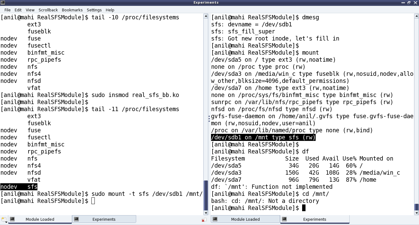
Figure 38: Bare-bone real SFS experiments
Pugs’ experiments (Explanation of Figure 38):
- Checked the kernel window /proc/filesystems for the kernel supported file systems
- Loaded the real_sfs_bb.ko driver
- Re-checked the kernel window /proc/filesystems for the kernel supported file systems. Now, it shows sfs listed at the end
- Did a mount of his pen drive partition /dev/sdb1 onto /mnt using the sfs file system. Checked the dmesg logs on the adjacent window. (Keep in mind, that right now, the sfs_fill_super() is not really reading the partition, and hence not doing any checks. So, it really doesn’t matter as to how the /dev/sdb1 is formatted.) But yes, the mount output shows that it is mounted using the sfs file system
Oops!!! But df output shows “Function not implemented”, cd gives “Not a directory”. Aha!! Pugs haven’t implemented any other functions in any of the other four function pointer structures, yet. So, that’s expected.
Note: The above experiments are using “sudo”. Instead one may get into root shell and do the same without a “sudo”.
Okay, so no kernel crashes, and a bare bone file system in action – Yippee. Ya! Ya! Pugs knows that df, cd, … are not yet functional. For that, he needs to start adding the various system calls in the other (four) function pointer structures to be able to do cool-cool browsing, the same way as is done with all other file systems, using the various shell commands. And yes, Pugs is already onto his task – after all he needs to have a geeky demo for his final semester project.