March | 2013 | Playing with Systems

This second article, which is part of the series on Linux device drivers, deals with the concept of dynamically loading drivers, first writing a Linux driver, before building and then loading it.

<< First Article

As Shweta and Pugs reached their classroom, they were already late. Their professor was already in there. They looked at each other and Shweta sheepishly asked, “May we come in, sir”. “C’mon!!! you guys are late again”, called out professor Gopi. “And what is your excuse, today?”. “Sir, we were discussing your topic only. I was explaining her about device drivers in Linux”, was a hurried reply from Pugs. “Good one!! So, then explain me about dynamic loading in Linux. You get it right and you two are excused”, professor emphasized. Pugs was more than happy. And he very well knew, how to make his professor happy – criticize Windows. So, this is what he said.

As we know, a typical driver installation on Windows needs a reboot for it to get activated. That is really not acceptable, if we need to do it, say on a server. That’s where Linux wins the race. In Linux, we can load (/ install) or unload (/ uninstall) a driver on the fly. And it is active for use instantly after load. Also, it is disabled with unload, instantly. This is referred as dynamic loading & unloading of drivers in Linux.

As expected he impressed the professor. “Okay! take your seats. But make sure you are not late again”. With this, the professor continued to the class, “So, as you now already know, what is dynamic loading & unloading of drivers into & out of (Linux) kernel. I shall teach you how to do it. And then, we would get into writing our first Linux driver today”.

Dynamically loading drivers

These dynamically loadable drivers are more commonly referred as modules and built into individual files with .ko (kernel object) extension. Every Linux system has a standard place under the root file system (/) for all the pre-built modules. They are organized similar to the kernel source tree structure under /lib/modules/<kernel_version>/kernel, where <kernel_version> would be the output of the command “uname -r” on the system. Professor demonstrates to the class as shown in Figure 4.

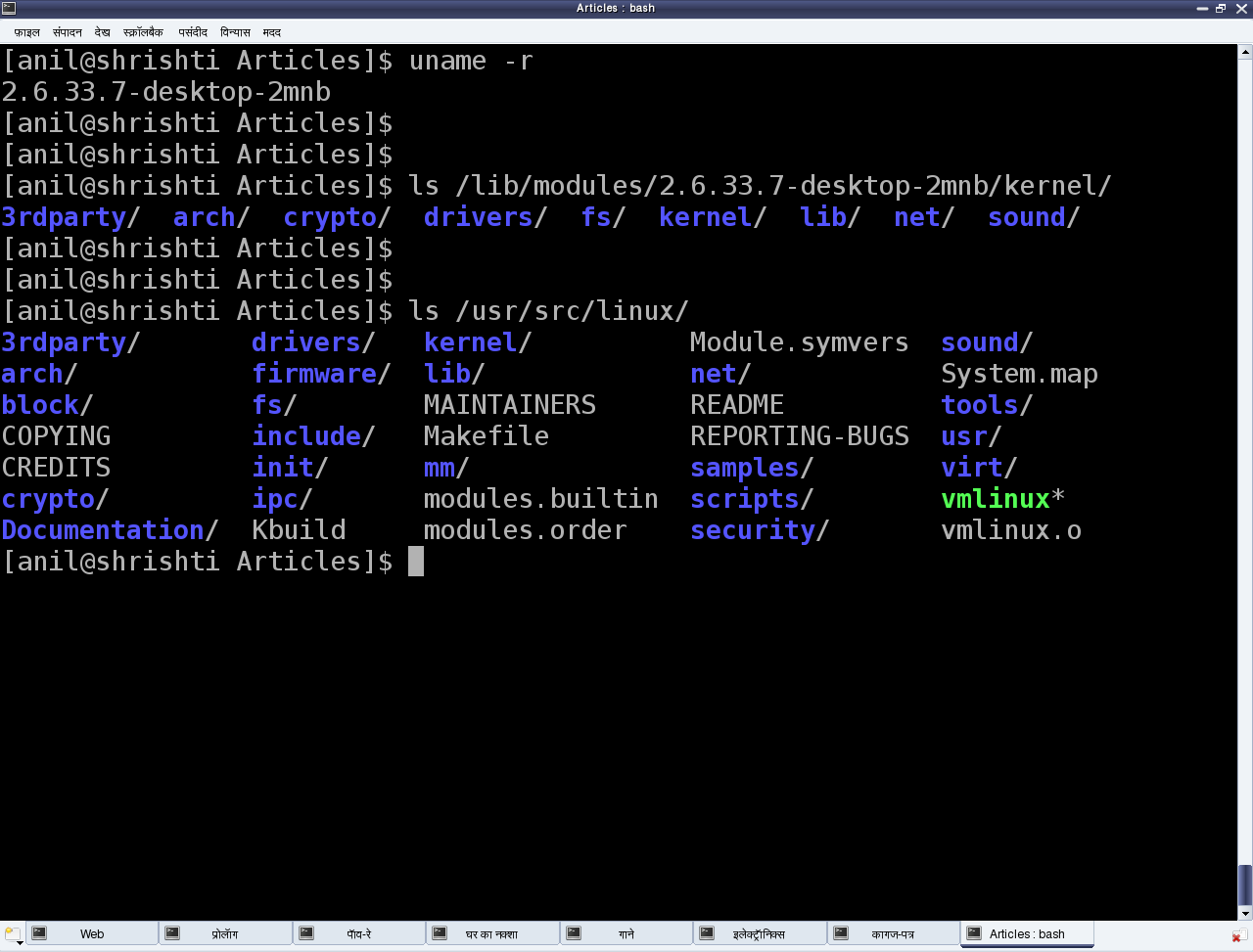
Figure 4: Linux pre-built modules

Now, let us take one of the pre-built modules and understand the various operations with it.

Here’s a list of the various (shell) commands relevant to the dynamic operations:

lsmod – List the currently loaded modules
insmod <module_file> – Insert/Load the module specified by <module_file>
modprobe <module> – Insert/Load the <module> along with its dependencies
rmmod <module> – Remove/Unload the <module>

These reside under the /sbin directory and are to be executed with root privileges. Let us take the FAT file system related drivers for our experimentation. The various module files would be fat.ko, vfat.ko, etc. under directories fat (& vfat for older kernels) under /lib/modules/`uname -r`/kernel/fs. In case, they are in compressed .gz format, they need to be uncompressed using gunzip, for using with insmod. vfat module depends on fat module. So, fat.ko needs to be loaded before vfat.ko. To do all these steps (decompression & dependency loading) automatically, modprobe can be used instead. Observe that there is no .ko for the module name to modprobe. rmmod is used to unload the modules. Figure 5 demonstrates this complete experimentation.

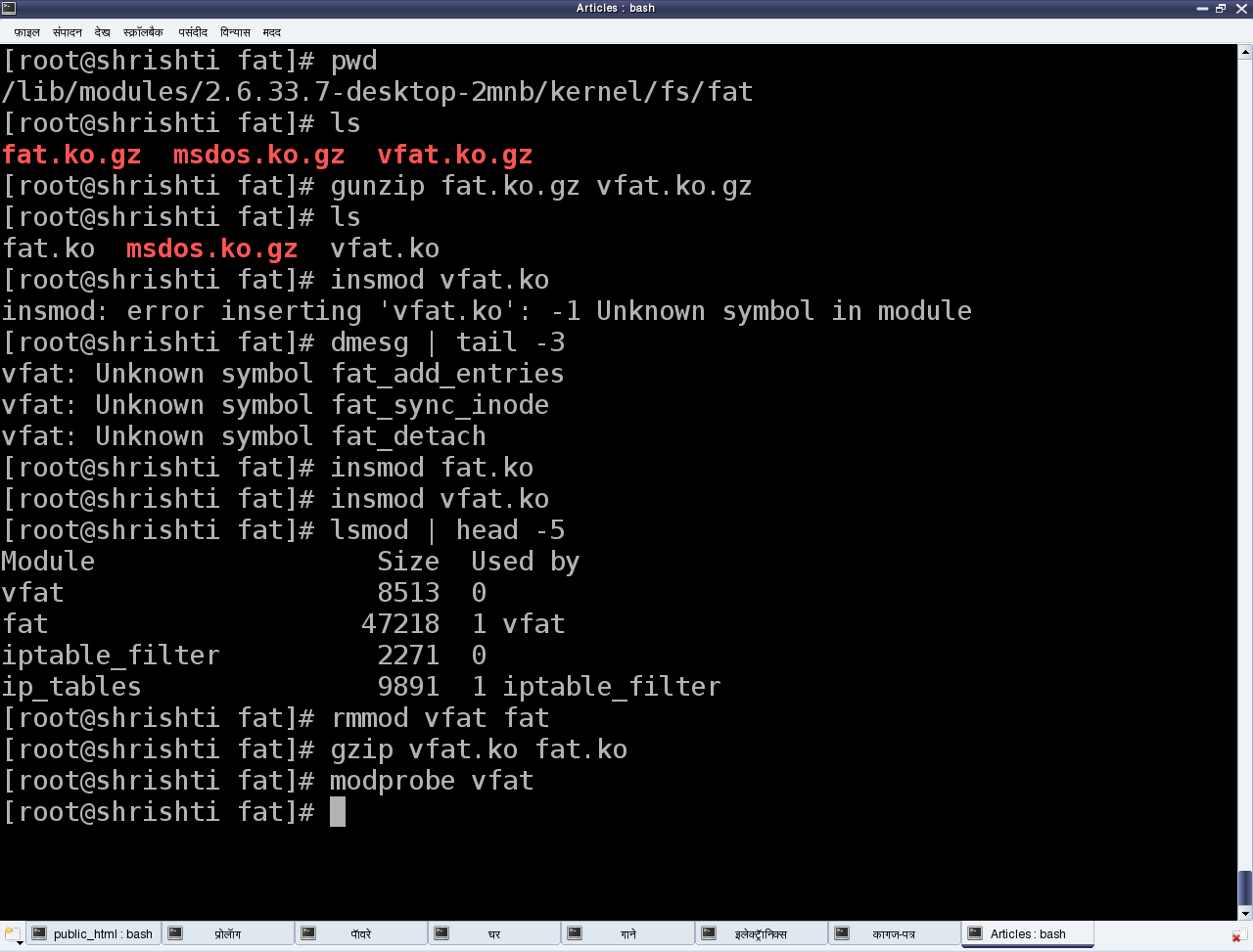
Figure 5: Linux module operations

Our first Linux driver

With that understood, now let’s write our first driver. Yes, just before that, some concepts to be set right. A driver never runs by itself. It is similar to a library that gets loaded for its functions to be invoked by the “running” applications. And hence, though written in C, it lacks the main() function. Moreover, it would get loaded / linked with the kernel. Hence, it needs to be compiled in similar ways as the kernel. Even the header files to be used can be picked only from the kernel sources, not from the standard /usr/include.

One interesting fact about the kernel is that it is an object oriented implementation in C. And it is so profound that we would observe the same even with our first driver. Any Linux driver consists of a constructor and a destructor. The constructor of a module gets called whenever insmod succeeds in loading the module into the kernel. And the destructor of the module gets called whenever rmmod succeeds in unloading the module out of the kernel. These two are like normal functions in the driver, except that they are specified as the init & exit functions, respectively by the macros module_init() & module_exit() included through the kernel header module.h

/* ofd.c – Our First Driver code */

#include <linux/module.h>
#include <linux/version.h>
#include <linux/kernel.h>

static int __init ofd_init(void) /* Constructor */
{
	printk(KERN_INFO "Namaskar: ofd registered");

	return 0;
}

static void __exit ofd_exit(void) /* Destructor */
{
	printk(KERN_INFO "Alvida: ofd unregistered");
}

module_init(ofd_init);
module_exit(ofd_exit);

MODULE_LICENSE("GPL");
MODULE_AUTHOR("Anil Kumar Pugalia <email@sarika-pugs.com>");
MODULE_DESCRIPTION("Our First Driver");

Above is the complete code for our first driver, say ofd.c. Note that there is no stdio.h (a user space header), instead an analogous kernel.h (a kernel space header). printk() being the printf() analogous. Additionally, version.h is included for version compatibility of the module with the kernel into which it is going to get loaded. Also, the MODULE_* macros populate the module related information, which acts like the module’s signature.

Building our first Linux driver

Once we have the C code, it is time to compile it and create the module file ofd.ko. And for that we need to build it in the similar way, as the kernel. So, we shall use the kernel build system to do the same. Here follows our first driver’s Makefile, which would invoke the kernel’s build system from the kernel source. The kernel’s Makefile would in turn invoke our first driver’s Makefile to build our first driver. The kernel source is assumed to be installed at /usr/src/linux. In case of it to be at any other location, the KERNEL_SOURCE variable has to be appropriately updated.

# Makefile – makefile of our first driver

# if KERNELRELEASE is not defined, we've been called directly from the command line.
# Invoke the kernel build system.
ifeq (${KERNELRELEASE},)
	KERNEL_SOURCE := /usr/src/linux
	PWD := $(shell pwd)
default:
	${MAKE} -C ${KERNEL_SOURCE} SUBDIRS=${PWD} modules

clean:
	${MAKE} -C ${KERNEL_SOURCE} SUBDIRS=${PWD} clean

# Otherwise KERNELRELEASE is defined; we've been invoked from the
# kernel build system and can use its language.
else
	obj-m := ofd.o
endif

Note 1: Makefiles are very space-sensitive. The lines not starting at the first column have a tab and not spaces.

Note 2: For building a Linux driver, you need to have the kernel source (or at the least the kernel headers) installed on your system.

With the C code (ofd.c) and Makefile ready, all we need to do is put them in a (new) directory of its own, and then invoke make in that directory to build our first driver (ofd.ko).

$ make
make -C /usr/src/linux SUBDIRS=... modules
make[1]: Entering directory `/usr/src/linux'
CC [M] .../ofd.o
Building modules, stage 2.
MODPOST 1 modules
CC .../ofd.mod.o
LD [M] .../ofd.ko
make[1]: Leaving directory `/usr/src/linux'

Summing up

Once we have the ofd.ko file, do the usual steps as root, or with sudo.

# su
# insmod ofd.ko
# lsmod | head -10

lsmod should show you the ofd driver loaded.

While the students were trying their first module, the bell rang, marking the end for this session of the class. And professor Gopi concluded, saying “Currently, you may not be able to observe anything, other than “lsmod” listing showing our first driver loaded. Where’s the printk output gone? Find that out for yourself in the lab session and update me with your findings. Moreover, today’s first driver would be the template to any driver you write in Linux. Writing any specialized advanced driver is just a matter of what gets filled into its constructor & destructor. So, here onwards, our learnings shall be in enhancing this driver to achieve our specific driver functionalities.”

Notes

In most of today’s distros, one may safely have KERNEL_SOURCE set to /lib/modules/$(shell uname -r)/build, instead of /usr/src/linux i.e. KERNEL_SOURCE := /lib/modules/$(shell uname -r)/build in the Makefile.

Third Article >>

Basic operations

For integer-only math, you may invoke the bench calculator as bc. For a full-fledged real number math, you may invoke it as bc -l. Once invoked, it will print a welcome message and then wait for you to just type your math statements and press Enter to get your answer. For quitting the bench calculator, you need to press Ctrl-D (^D), on an empty line. All the basic arithmetic operations: addition (+), subtraction (-), multiplication (*), quotient (/), remainder (%), power (^), brackets (()) are just there – with the C-like precedence & associativity rules. An example with all of them in use:

$ bc bc 1.06.95 Copyright 1991-1994, 1997, 1998, 2000, 2004, 2006 Free Software Foundation, Inc. This is free software with ABSOLUTELY NO WARRANTY. For details type `warranty'. 2 + 2 * 3 - 5 + 21 / 4 * 6 # A basic maths statement 33 (2 ^ 2) ^ 3 # Another one with power & bracket 64 ^D

Yes, you guessed it right. # starts a one-line comment as in shell, or like // in C++. For a multi-line comment, you may use /* */ as in C/C++. You may want that in case you are writing a complete program in bc. Yes, you can even do that. How? You may put your math statements (each one on a line by itself) in a file, say in prog.bc, as follows:

2 + 2 * 3 - 5 + 21 / 4 * 6 # A basic maths statement (2 ^ 2) ^ 3 # Another one with power & bracket quit # This will complete the program and not wait for more input

And then execute – yes I mean execute, you do not need to compile it – as follows:

Aha! You actually got the welcome message from bc and then your results. To avoid the welcome message, you may add -q option to bc, as follows:

$ bc -q prog.bc 33 64 $

You may also try out the difference in the output of the same program with a -l option, i.e. with real numbers. Then, / would be treated as a complete division, not just a quotient provider. Here’s what you would get:

$ bc -ql prog.bc 34.50000000000000000000 64 $

Programming with bc

As soon as we say programming, the first thing flashing to your mind might be variables. Yes, so they are there. All the variables must start with a small letter alphabet and then may contain numbers or small letter alphabets. Yes, you read it right – only small letter alphabets (a,b,c,…,z). This is because, capital letters (A,B,C,…) are used to represent numbers in other bases greater than 10. Yes, bc have support for various bases from 2 to 16, and two variables associated with them: 1) ibase: defines the base for input; 2) obase: defines the base for output. By default, both are set to 10, as in our day-to-day usual maths. But can be modified, for more fancier base conversions. Here’s a snippet:

$ bc -ql ibase # Show the current input base 10 obase # Show the current output base 10 obase=16 # Set the output base to 16 108 # Input in base 10; Output should be in base 16 6C obase=10 # Set the output base back to 10 ibase=16 # Set the input base to 16 11 # Input now in base 16; Output should be in base 10 17 ibase=10 # Set the input base to 16. 10 is 16 in input base 16. ibase=A # Set the input base to 10. obase=2 # Set the output base to 2, i.e. binary x = 2 * 5 - 1 # Set the variable x to 9 (input base 10) x # Display the value of x (in output base 2) 1001 x * 2 # This should display 18 in base 2, but x is still 9 10010 obase=10 x++ # Post increment: Display the current value of x and then increment it 9 x # Display the incremented value 10 --x # Pre decrement: Decrement x and then display its value 9 ^D

From the demo above, you might have already observed that there is nothing like declaring variable type or so – just assign them using = and then use them. Moreover, bc also have basic conditional and loop constructs: if, for, while, break, continue. And along with are the usual C-like relational (<, <=, >, >=, ==, !=), logical (!, ||, &&), and the operation-assignment (-=, +=, *=, /=, %=, ^=) operators. Note of caution: Their precedence and associativity rules may not be as in C. If you do not understand that, forget about it – just make sure to use brackets for whatever you want to operate first. Here goes two simple programs to demonstrate: 1) Computing the sum of the first n numbers (sum.bc); 2) Computing the product of the first n numbers, i.e. factorial of n (factorial.bc)

-------------------------------- file: sum.bc ----------------------------- print "Enter a positive number: " num = read() sum = 0 current_num = 1 while (current_num <= num) { sum += current_num current_num += 1 } print "Sum of first ", num, " numbers is: ", sum, "\n" quit

-------------------------------- file: factorial.bc ----------------------------- print "Enter a positive number: " num = read() product = 1 for (current_num = 1; current_num <= num; current_num += 1) { product *= current_num } print "Product of first ", num, " numbers is: ", product, "\n" quit

The above programs can be tried out by issuing shell commands bc -ql sum.bc and bc -ql factorial.bc, respectively. But, what are those two words: print & read, doing there in the code. What else; they are just two built-in functions, displaying the message to the user and taking a number from the user, respectively. Functions? Yes, bc can do functions as well. That’s what would be our next camping. So, right now, just go ahead and try the above programs.

Playing with Systems

SysPlay's Blogs

Monthly Archives: March 2013

Writing your First Linux driver in the Classroom

Dynamically loading drivers

Our first Linux driver

Building our first Linux driver

Summing up

Notes

Explore the Power of the Bench Calculator

Basic operations

Programming with bc