Toolchain Setup

This is the third article in the series dedicated to the world of Embedded Systems.

<< Previous Article

“Shall we meet now to further our discussion?” was a text on Pugs’ mobile.

“Where?”, asked Pugs.

“Office Park”, was the reply back from Shweta.

I’ll be there in another 5 minutes.

In the park, “No-thanks, for your time”, were the first words from Pugs.

You won’t change.

Do you want me to?

“Let’s come to the topic – toolchain”, was a change of topic from Shweta, while opening her laptop. “So, your question was, why different toolchains, for different embedded types (BS or OS based), even if they are for same architecture”, she continued.

Wow! You remember my doubt.

Now, to understand that, let me first tell you a bit about the nomenclature (naming conventions) of the toolchain prefix. A native toolchain will have commands like gcc, as, ld, objdump, etc. However, as soon as it is a cross toolchain, a cross compile prefix is prefixed with all these commands as <prefix>-gcc, <prefix>-as, <prefix>-ld, <prefix>-objdump, etc

Yes Yes. I know, e.g. arm-linux-gnueabihf- is prefixed to provide commands like arm-linux-gnueabihf-gcc, arm-linux-gnueabihf-as, etc.

Yes. But the prefix is not random, it is derived based on some naming convention.

O really! What is it?

The prefix is typically created using the following format: <arch>-<vendor>-<os>-<abi>-, where <arch> represents the architecture for which the toolchain would generate the code, <vendor> would be the vendor who created the toolchain, <os> would be the operating system for which the toolchain creates the executable, <abi> denotes the application binary interface (ABI).

What is this application binary interface?

It is an understanding or protocol of interfacing / communicating between the C code (application), and the assembly / machine code (binary). As examples of this protocol, in which CPU register or how in stack would the corresponding parameters of a C function would be placed, where would the return value of a function be placed, floating point computations would be hardware based or in software, etc.

Okay. So, you mean to say, depending on the toolchain, this understanding may also change.

Yes. That’s why, you typically need to compile all software used together with the same toolchain. Examples of ABI are Embedded ABI (EABI), GNU’s EABI (gnueabi), GNU, ELF, etc. And if they incorporate hardware based floating point operations, an “hf” may be suffixed, e.g. gnueabihf.

Hmmm. Examples of <arch> in the prefix would be arm, aarch64, armv8l, etc, right?

Yes. And <os> could be linux or none, if it is for baremetal.

<vendor> could be linaro, right?

Yes. However, in the prefix, many a times the <vendor> is omitted. And even <os> could be omitted if it is none.

Wonderful. So, just by observing the prefix of the commands in a cross toolchain, we can deduce many things about it.

Yes. Just check out some examples here: https://releases.linaro.org/components/toolchain/binaries.

There are so many versions here. Which one?

Say 6.5-2018.12. So, go to: https://releases.linaro.org/components/toolchain/binaries/6.5-2018.12, and you’ll see the following:
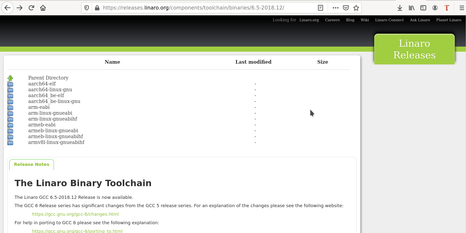
Toolchain List

Yes. I see there are 3 ARM related toolchains. arm-eabi must be for baremetal, and arm-linux-gnueabi* are for Linux based builds – one with soft float and one with hard float gnueabi.

Excellent. Now, each one of them is available for various host systems – systems where we are going to run the toolchain. As my system is a 64-bit Linux system, I’ll download & install the corresponding arm-eabi and arm-linux-gnueabihf toolchains. One may choose other options in case of different host systems.

Why did you choose two toolchains?

You only wanted, to understand why two different toolchains for the BS and OS based embedded systems, right? So, I’ll setup both and then show you the differences by experimenting with them. And that would answer your question.

Okay. Okay. But, these are tar files, right? How to install?

Just untar them, say under /opt, as follows:

$ sudo tar -C /opt -xf gcc-linaro-6.5.0-2018.12-x86_64_arm-eabi.tar.xz
$ sudo tar -C /opt -xf gcc-linaro-6.5.0-2018.12-x86_64_arm-linux-gnueabihf.tar.xz

And then add their executables’ paths in the PATH variable, by adding the following lines in ~/.profile or ~/.bash_profile (as appropriate):

export PATH=~/GIT/bbb-builds/Downloads/gcc-linaro-6.5.0-2018.12-x86_64_arm-eabi/bin:${PATH}
export PATH=~/GIT/bbb-builds/Downloads/gcc-linaro-6.5.0-2018.12-x86_64_arm-linux-gnueabihf/bin:${PATH}

I guess in debian based systems like Ubuntu, we need to add in ~/.profile, and in other rpm based systems in ~/.bash_profile.

Typically, yes.

But these profile files get sourced only when we login, right?

Yes. And so, now after doing the above, I am logging out.

With that Shweta does a logout in her laptop, and then does a login back.

“Now see, the various commands are available on the konsole”, Shweta continued, while showing her screen, after typing arm- and pressing the tab key on her konsole:
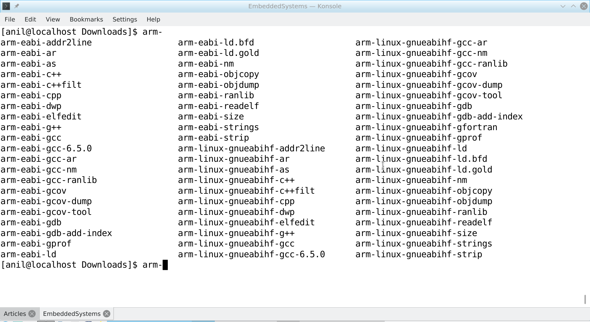
Toolchain Commands

Good. Now, like I use gcc and other commands, I can just use these instead.

Yes. With this, we are all set to use the two toolchains, which I’ll use on a simple C program to demonstrate you the differences between the two toolchains, which will clarify “why two”. Meanwhile, why don’t you get your laptop and set it up, to explore alongwith me.

O Yes! That’s a good idea. Let me get it.

With that, Pugs’ goes to fetch his laptop.

   Send article as PDF   

Toolchain over a Cup of Coffee

This is the second article in the series dedicated to the world of Embedded Systems.

<< Previous Article

“Wow! You are already there”, pulled Shweta on Pugs.

“Has to be. As an obedient student, how can I keep my guru waiting for me”, was a naughty reply from Pugs.

Okay. Ok. So, what were we discussing about?

Two categories of Embedded Systems.

O yes! Baremetal Software (BS) based, and Operating System (OS) based. In BS based embedded systems, the firmware is the only software component. It has its own pros & cons. As being the minimal software, it typically yields better control of timing & performance. But the downside is that it is a development from scratch. Everything and anything needed has to be designed and developed – no software logic can be assumed to be there.

Wow! That would be amazing, right? One would get a feel of the days, when the first software was written.

Similar to that. But not exactly. As when the first software was written, it was written directly using the CPU instructions aka machine codes.

Yes. Yes. Nowadays, we write in C, or other higher level languages.

Yes. But even then, it ultimately needs to get converted into machine codes. So, for that we would use a compiler.

Yes that I know. But what is a cross compiler?

See in general, you run a compiler on your x86 desktop to generate the machine code for your x86 system only, i.e. you compile the code for your native system itself. However, embedded systems typically have non-x86 architectures like ARM, PPC, MIPS, etc. But we still wish to compile the code for them on our desktops, instead of compiling it on the embedded system.

Why is that so?

Because of the usual embedded system restrictions, and ease of development on our familiar desktops. In such scenario, we need to have a compiler which runs on a x86 system (typically referred as a host system), but generates the machine code for a non-x86 system (typically referred as a target system). And such compilers are called cross compilers.

So, a compiler where the host and target are not same is called a cross compiler.

Exactly.

So, say I am somehow able to do compilation for my ARM based target system, on the target system itself. Then, wouldn’t it be a cross compiler?

Yes, it wouldn’t be – it would be just an another native compiler, though ARM based. As then, your compiler would run on an ARM system and generate code for the same system. And why somehow? When you have a complete Linux distribution running on an Embedded System, you can easily have the ARM based native compiler in there.

Got it. Then, what is this so called (cross) toolchain all about?

When we talk about a (cross) compiler, we are referring to a single software (tool) that converts say C into machine code. But typically to do that there are many other related tools, which are used, like an (cross) assembler, (cross) linker, etc. Moreover, there are many other related utilities, which are useful in development, like (cross) objdump, (cross) nm, etc, grouped together as binary (lowest level output) manipulating utilities aka (cross) binutils. All these set or chain of tools put together is called a (cross) toolchain.

O! That’s all – just for the name of a toolchain.

It’s not, that’s all. A toolchain is a topic in itself. Developing a specific toolchain involves many things, and multiple iterations. Just to give you an idea. Toolchain is after all a software. So, what do you think it is written in?

C, I guess.

Nowadays, yes. So, we need to have a toolchain, to compile a toolchain.

That’s okay. We may use other already built toolchain, right?

Not that straight forward. There may incompatibilities with that. As a toolchain consists of a set of libraries, OS dependent headers, etc, which may be different for different versions.

So, what do we do then?

We first build a minimal version independent toolchain using an existing toolchain, and then use that to build the complete toolchain.

Interesting.

And involved.

But then, how would have been the first toolchain built?

Possibly using a C compiler not written in C, but assembly.

And that would have been assembled using an assembler. And then continuing down further, the first assembler would have been written in machine code itself.

Excellent.

That’s why. Rather than building toolchain ourselves, we typically, get these ready-made from some websites, right?

Yes but they are not just websites, rather full-fledged companies built around toolchains. For example, Linaro.

Makes sense.

However, there are full-fledged build systems to build complete Linux distributions, like buildroot, yocto, etc, which in turn build their own toolchains in an automated fashion, taking care of all the complications involved.

Wonderful. Based on our discussion, what I understand is that irrespective of the embedded system type (BS or OS based), we would need a toolchain for its software development. And it is upto us, whether we download the pre-built ones, or build ourselves – manually or preferably using build systems.

Yes. But depending on the type, the toolchain may vary. And note that the build systems may be able to generate the toolchain only for an OS based embedded system.

“Yes, I can see there are broadly two types of toolchains on the Linaro website”, quipped Pugs browsing the above link. “But why do they need to be different. Finally, they are going to be generating the machine code for the same architecture – isn’t it?”

I need to go now. Some other time on that.

When?

I’ll message you.

Next Article >>

   Send article as PDF   

Embedded Systems for your Boy Friend

This is the first article of the series dedicated to the world of Embedded Systems.

<< Previous Story

“Hey Pugs!”, was a slow whisper from Shweta from her cubicle.

“Shweta!!!”, was the only word which came out of Pugs, as he turned around in the aisle.

“What a surprise! After so long! How come you are here?”, came out a burst of statements from Shweta. It was not unexpected, as she has seen Pugs after a long gap of 6+ years, since they have graduated out from the college.

“How … how come you are here?”, stumbled out some words from Pugs.

What “how come”? I work in this office. What about you?

I just joined today, and HR was just taking me around.

Great! I don’t have words to express my feelings seeing you after so long. Do you mind if I take you around, rather?

I don’t have one to mind.

Pugs, you haven’t changed a bit.

You too look the same.

Thus went on, a seemingly unending chat between the duo, while strolling in and around the office.

And then, “What are you working on?”, asked Pugs.

Embedded Systems.

Wow! Where do you embed the systems into?

Are you joking?

Not really. I have been majorly working in the desktop world. Heard about this and other related jargons. But not really very clear about what really it is all about so called “Embedded Systems”. So, could you please teach me?

That was surely a joke. I remember our college days, how I used to learn from you.

So what? Knowledge and Learning knows no gender, time, and place. Anyone can teach. Anyone can learn. Whenever they want. Wherever they want. So, you are my Embedded Systems mentor.

Okay, dude – as you wish – you haven’t stopped giving gyaan. So, as such, any hardware system which is intended to do a specific task, or a specific set of tasks(, with some software embedded in there) can be called as an Embedded System.

You mean to say my hand watch, cafeteria’s micro wave oven, this printer, etc are all embedded systems, as they are meant to do their pre-designated specific tasks.

In a way, yes. Also, typically when we refer to something as an embedded system, it implies that it has some kind of software embedded in there as well.

Hmmm! And that is where the name “Embedded Systems” comes from. So, if it is purely hardware like the watch, then we may not call it an embedded system, right?

Traditionally yes. But nowadays the line has become so thin, that even a system seemingly to be a pure hardware system, has some software (embedded) in it, in some form or the other. For example, your watch itself is not a pure hardware – it has enough software to say, sync it with your mobile.

I see. So, what about the mobile phones? Can we call them embedded systems? They have both hardware and software. But they are not meant for any specific tasks. They are like a desktop only.

In its initial evolution, a mobile definitely used to fit in the above mentioned definition of an embedded system – hardware plus software meant for specific task, as it was specifically meant for telecommunication only. But as the world of such embedded systems evolved, the definition also evolved to encompass a wider variety.

And with this new definition, can mobile phones be still called embedded systems?

Yes.

I know. In this expanded definition, any hardware plus software system which needs to operate under constraints of limited resources is called an embedded system.

Correct. Now, how do you know this?

I keep reading many articles around. But now I have a doubt. Nowadays, we see that even such constraints are possibly going away with embedded systems having huge memories, powerful processors, etc, comparable to the desktop world. So, should they be still called embedded systems?

Even with those, don’t forget that, at the least, the constraint of miniaturization is day by day increasing only. Hence, this current definition should be good enough for at least some more time to come.

That seems reasonable. Now, when you say all embedded systems have some kind of software in it, I assume it need not be an operating system based one, right?

Yes. In fact, it can’t be. As many such systems have very limited memory and storage, not enough for an OS. And that is where, all embedded systems can be broadly classified into two categories:

  • Baremetal Software based, i.e. the ones without the Operating System
  • Operating System based, i.e. the ones with the Operating System whether RTOS, or a full-fledged one

RTOS meaning Real Time Operating System, right?

Yes.

What is then this so called “Firmware”?

The baremetal software, i.e. the software in the OS-less systems is often referred to as “Firmware”.

Oh I see! So much for that jargon. You have just de-jargonified it for me. No thanks to friends.

Good to hear that.

Can you also give me an overview of the software development process in these two categories of embedded systems – with and without OS?

Sure. But not now. I need to finish some of my work. How about discussing that over a cup of coffee?

My pleasure.

Next Article >>

   Send article as PDF   

Poisoned Dish

<< Previous Article

There are very many puzzles around, involving binary choices, or so called yes-no, true-false, … situations. Here is one such.

Puzzle #3: There was a king who got 1001 identical dishes prepared for his 1000 guests and himself. But one hour before the guests were to arrive, he was informed that out of the 1001 dishes, one has got poisoned. And whoever even tastes it would die in an hour. Moreover, which dish is poisoned was not known. Now, the king has few taster slaves, who could be made to taste the dishes, and figure out which dish is poisoned. But the problem is they were only few, not 1001. So, the question is what is the minimum number of taster slaves required to figure out the poisoned dish?

As usual, think through before you peek into the solution.

Here are some hints, if you have tried for some time.

Note that the outcome of tasting a dish is binary – the taster either dies or doesn’t die.

Work on some pattern in deciding who should taste which dish.

Number the dishes from say 0, 1, …, 1000.

Think. Think.

Ok. Got it. Good. Not yet. What if there are only 10 taster slaves? Can it be solved?

That’s more than enough hints.

By now, you might have at least tried various combinations, say like arranging 1000 dishes in an 10 x 10 square, and making n’th slave taste all dishes in n’th row and n’th column etc. If not, go ahead and try it.

And here’s finally one way of doing it.

Number the 1001 dishes from 0 to 1000, but in binary using 10 bits, as 10 bit can represent numbers from 0 to 1023. So, the numbering would be like 0000000000, 0000000001, …, 1111101000. Then, label the 10 taster slaves from 0 to 9. Now, let the i’th slave taste all the dishes, the binary representation of which has a 1 in its i’th bit position. After one hour, note down the labels of all the taster slaves which die. Create a 10-bit binary number with all its bit positions corresponding to those labels, set to 1. Now, whichever dish has the number matching with this created number, is the poisoned one.

Does it make sense? If not, please ping in the comments.

If you have got any other interesting way of solving it, then also please share it in the comments.

   Send article as PDF   

Weighing Stones

<< Previous Article

Puzzle #2: A 40 kg stone was being delivered to a shopkeeper. On the way, it broke into 4 pieces. When he received them, rather than becoming angry, he was happy after analyzing them. Onlookers asked, “How are you happy even after this loss?”. To that, he replied, “Now these four pieces would be useful for me in an another way. I can use them with my beam balance to be able to weigh goods of all integral denominations from 1 to 40 kgs.”

So the question is, what are the individual weights of the four pieces of the 40 kg stone?

Like Puzzle #1, this also could be solved in many ways. Try solving it yourself before proceeding further to see the analysis.

The first attempt typically done to solve any puzzle is basically to understand the puzzle, by trying to observe and register some patterns about it. Same here. Say first piece is 1 kg. Second one is 2 kgs. Then, 3 kgs could be weighed using these two. So, say the third one is 4 kg. Then, 1 + 4 = 5, 2 + 4 = 6, 1 + 2 + 4 = 7. But then, we can’t get 8 etc as the fourth piece would be 33 kgs (= 40 – 1 – 2 – 4). So, seems like 1, 2, 4 must be even more apart. O! Just hold on. In a beam balance, we can weigh not only by placing weights on one side, but on either, and moreover on both sides. For example, placing 1 kg on one side, 4 kgs on the other side would also weigh 3 kgs. Ok. Let’s restart. Say, first piece is 1 kg. Let second be 3 kgs, as 3 – 1 would anyways be able to weigh 2 kgs. Note that, making the second one as 4 kgs may not be okay, as then how do we weigh 2 kgs. Now, 1 + 3 = 4. So, for the third piece, a way could be to get 5, when the first two are subtracted from it. That is, X – (1 + 3) = 5. Then, the third one would be 9. 9 – (1 + 3) = 5, 9 – 3 = 6, 9 – 3 + 1 = 7, 9 – 1 = 8, …, 9 + 3 + 1 = 13. That seems interesting, as just with three pieces, upto 13 kgs have been achieved. But then the fourth piece would be 27 kgs (= 40 – 1 – 3 – 9). Would that serve the purpose? Check it out. Is there any pattern? Post your comments.

Now, the idea of looking into such puzzles, is not to stop after solving them. But how can these be generalized. What is the maximum weight till which all integral denominations could be weighed if there were 5 pieces of any desired individual weights? And why 5? What if it is any “n”? Can we get an answer to it? If there is a pattern, it is highly likely to get a generalized solution for any “n”. Think through it, and you’ll be amazed.

Programmers rather prefer to think in terms of programming, to solve any problem at hand, even if it is a puzzle. So, what do you think? How can it be solved programmatically? Again, don’t jump to “n”. Let’s start with the initial 40 kg stone problem itself. And once we get an idea, it could be generalized.

One approach could be to generate all 4-tuples (a, b, c, d), such that a + b + c + d = 40. We may further restrict that all of a, b, c, d are distinct. And then for each such tuple, we may check, if all integral denominations upto 40 kgs can be weighed using them. How do we check? For that, all the different placement combinations for a given tuple (a, b, c, d) have to be tried. What are the possibilities? 3 possibilities per piece: 1) Do not use it, 2) Put it on the left side of the beam balance, 3) Put it on the right side of the beam balance. Seems like 3 * 3 * 3 * 3 = 3^4 = 81 possibilities for all the 4 pieces. Not bad. It definitely can be tried using a program. Go ahead. Give it a try. You may start with an empty array of 40 elements. And keep marking, which ever weight has been achieved by any of these combinations. At the end of trying all combinations for a particular tuple, if we have been able to mark all 40 elements of the array, then the tuple is definitely one of our possible solutions.

What if we remove the particular case of not selecting any of the 4 pieces, then total combinations are 80 (= 81 – 1). And the remaining 80 are actually duplicated, e.g. putting “a” alone on left side is same as putting it alone on right side of the beam balance, and so on. So, there would be actually only 40 (= 80 / 2) unique combinations. O! That seems to hint towards the possibility of achieving all integers 1 to 40.

This is just one thought. Obviously, other interesting thoughts may be applied. And that’s the intention of this writing. Please put it down in the comments to trigger further discussions. Who knows? You may come up with an optimal algorithm.

Next Article >>

   Send article as PDF   

Magical Pond

<< Previous Article

Decoding and solving puzzles has been there since very early days of mankind. And that has played a crucial role in the evolution of human brain. In the beginning, nature alone used to throw up puzzles for human brain to solve, for its mere existence itself. However, as human brain became more refined in thinking, analysis, and logic, it started creating its own puzzles, as well. So, today we have man-made puzzles and riddles as well, though many a times inspired from real life scenarios. Thus, inspired by the important role of puzzles in human life, and how have they been approached and solved in different ways, here is an attempt to present a semi-formal approach of logic analysis and problem solving in decoding puzzles. It would be attempted by picking up various sets of puzzles.

Puzzle #1: There is a square-shaped magic pond, which doubles the flowers dipped into it. On the four corners of the pond are four temples. A devotee comes with some flowers. She dips them in the pond. Flowers get doubled. Then, she offers some of those flowers in the first temple. She then again dips the remaining flowers in the pond. Flowers again get doubled. She then offers the same number of flowers in the second temple, as she offered in the first temple. Again the remaining flowers are doubled, and the same number of flowers are offered in the third temple, as in the second temple. And finally, the remaining flowers are doubled for the last time, and all of them are offered in the fourth temple. Interestingly, the number of flowers offered in the fourth temple is also same as that in the third temple. So, what is the minimum number of flowers the devotee would have brought, and what is the number of flowers offered in each temple?

Now, there could be many approaches to solve this puzzle. Try solving it yourself before proceeding further to see the analysis.

The first attempt typically done to solve any puzzle is basically to understand the puzzle, by trying to observe and register some patterns about it. Same here. So, one would start trying with some numbers. Say she came with 1 flower, doubled it to 2, then offered 1, and continued so forth till fourth temple. But then, if the fourth temple is also offered with 1 flower, she would have 1 flower remaining with her. So, seems like the number of flowers brought and offered can’t be same. On further delving, there would be a realization that flowers offered need to be more than flowers brought, for it to reduce on consecutive iterations. Moreover, the flowers offered need to be less than twice the flowers brought, for the same reason. Given this understanding, one may try with next set of possible numbers as 2 flowers brought and 3 flowers offered. Not working. Then, with 3 flowers brought, either 4 or 5 flowers could be offered. Interestingly, with 3 flowers brought, and 4 flowers offered, all flowers get over in the second temple itself. And with 1 flower brought, and 2 flowers offered, all flowers were getting over in the first temple itself. Wow! There seems to be some pattern.

Now, one can approach this way, and finally get a solution. But as this is a trial and error kind of approach, computers are better in solving this. And a programmatic flow can be evolved for the same. And in that case, why only for a square pond? Why not an n-sided polygon pond with n temples? Great idea. And here is how the logic for that could be laid out:

solved = false;
brought = 1;
while (!solved)
{
	for (offered = brought + 1; offered < 2 * brought; offered++)
	{
		if (solved = solve(n, brought, offered))
		{
			printf("Min Brought: %d. Offered: %d\n", brought, offered);
			break;
		}
	}
	brought++;
}

where the solve() function could be the puzzle iterator, as follows:

solve(n, brought, offered)
{
	rem = brought;
	for (i = 1; i <= n; i++)
	{
		rem = 2 * rem - offered;
	}
	return (rem == 0) ? true : false;
}

Why is the minimum number of flowers brought, is being discussed? This can be easily seen by replacing the while (!solved) by a while (1). And there would be a continuous listing of infinite solutions to this puzzle.

Furthermore, why does the magic pond only double? What if it makes it k-times? The above problem could be parameterized even for that to observe even more interesting patterns – left as an exercise for the reader.

Now, this was just one approach to solve the puzzle and without any hesitation could be called as the computer science approach.

What if one wants to do it without computer science fundae – computer science is only very recent, right? Yes, as mentioned earlier, there could be many more approaches to the problem. Computer Science is just an ease. Or, rather an approach of making ourselves easier by trying to offload our brain tasks to computers.

Just to demonstrate that there could be other approaches as well, one may take a mathematical approach using algebra to solve the same. Let ‘b’ be the (positive) number of flowers brought, and ‘o’ be the (positive) number of flowers offered. Then, using these two variables, one may form an equation as per the puzzle, and then solve it. It would turn out to be one linear equation in two variables, and hence offering infinite solutions, same as above.

Expecting an answer to the above puzzle. Just try it out and find out for yourself. And may be, using your own approach. And then don’t forget posting it below in the comment box.

Next Article >>

   Send article as PDF   

Magic Square

<< Previous Article

A magic square is a square, with n rows and n columns, and thus consisting of n2 smaller squares. Moreover, each of these squares are filled with a distinct number, such that the sum of all the numbers in a row is equal to the sum of all the numbers in any other row or column. If n is even, it may not be always possible to form such a magic square, e.g. there exists no magic square for n = 2. However, if n is odd, there are infinitely many magic squares possible for all such n. To restrict this infinitely many to a finite number, the n2 squares are typically filled with the consecutive numbers 1, 2, …, n2. Once a magic square is obtained using these numbers, then by adding any integer to all of the squares, one may obtain yet another magic square. And thus, as integers are infinite, there is an infinite number of possible magic squares for a given n.

Interestingly enough, for an odd n, there exists a simple logic to fill the numbers 1, 2, …, n2 into a n x n magic square. Consequently, the sum of any row or column turns out to be n * (n2 + 1) / 2. And the middle most number turns out to be (n2 + 1) / 2. Here is the logic to fill the numbers 1, 2, …, n2, in that order:

  • Fill 1 in middle most square of the first row
  • For every next number, follow the steps below:
    • If the current number is filled in the first row, then fill the next number in the last row, in the column just next to the current one. If it is not applicable or possible, follow the next step.
    • If the current number is filled in the last column, then fill the next number in the first column, in the row just above the current one. If it is not applicable or possible, follow the next step.
    • Fill in the row just above the current one in the just next column. If it is not applicable or possible, follow the next step.
    • Fill in the row just below the current one in the same column. If all the above fails, this will be always possible.

In a more programmatic format, it would look like this, assuming the magic square to be a 2-D array of size n x n, with its index starting from 0:

magic_square(int M[n][n])
{
	r = 0; // current row
	c = (n - 1) / 2; // current column

	for (i = 1; i <= n * n; i++)
	{
		M[r][c] = i;
		if ((r == 0) && (c < (n - 1)))
		{
			nr = n - 1;
			nc = c + 1;
		}
		else if ((c == (n - 1)) && (r > 0))
		{
			nr = r - 1;
			nc = 0
		}
		else if ((r > 0) && (c < (n - 1)))
		{
			nr = r - 1;
			nc = c + 1;
		}
		else // ((r == 0) && (c == (n - 1)))
		{
			r = r + 1;
			c = c;
			continue; // as this is always possible
		}
 		if (!isfilled(M[nr][nc]))
		{
			r = nr;
			c = nc;
		}
		else
		{
			r = r + 1;
			c = c;
		}
	}
}

On a closer observation, the statements in the first three conditionals of the first if … else above are identical with modulo n (% n), i.e. they are same as:

nr = (r - 1 + n) % n;
nc = (c + 1) % n;

and the logic of the last else in both the above if … else are identical.
Hence, the logic can be further compacted as follows:

magic_square(int M[n][n])
{
	r = 0; // current row
	c = (n - 1) / 2; // current column

	for (i = 1; i <= n * n; i++)
	{
		M[r][c] = i;
		nr = (r - 1 + n) % n;
		nc = (c + 1) % n;
 		if (!isfilled(M[nr][nc]))
		{
			r = nr;
			c = nc;
		}
		else
		{
			r = r + 1;
			c = c;
		}
	}
}

Here’s 5 x 5 magic square to understand the above logic:

17 24 1 8 15
23 5 7 14 16
4 6 13 20 22
10 12 19 21 3
11 18 25 2 9

Next Article >>

   Send article as PDF   

Naturally Recursive Trees

<< Previous Article

A tree is one of the many data structures, which is naturally recursive, i.e. recursive by its design itself. A tree is made up of a so called “root” node, which has zero or more (sub)trees hanging from it, and each node would have some data &/or attributes associated with it. The subtrees give the natural recursion of lower order. And because of that, all the operations on a tree, starting from creation, can be done recursively.

A good example to understand this notion of recursion in trees is a (integer) binary search tree (BST). A (integer) binary tree is a tree with all its nodes having a maximum of two subtrees hanging from them(, and containing integer data). It would become a binary search tree, if data among all its nodes is unique, and the following conditions are satisfied for every node:

  • Every data in the node’s left subtree (if any) is smaller than node’s data
  • Every data in the node’s right subtree (if any) is greater than node’s data

The advantage of such a construction is that once the tree is created from say N given data points, searching for a specific data point, in those N data points, is very optimal – takes only log2(N) steps on an average. And that’s where the name binary “search” tree also comes from. And interestingly enough, if the tree is traversed in an inorder way, i.e. in the order of left subtree (if any), node itself, and then right subtree (if any), the data so obtained would be in the ascending sorted order.

Let B denote the binary search tree, and v any data value. Also, let B->left, B->data, B->right be the left subtree, data of the root node, right subtree, respectively of the binary search tree B. Then, the various operations of the binary search tree may be depicted recursively by recursing on the left & right subtrees, and with the actual operation in the terminating condition.

Inserting a value v in the BST B:

bst_insert(B, v) // only if v is not already there in B
{
	if (isempty(B))
	{
		setup(B); // With empty B->left and B->right
		B->data = v;
	}
	else if (v < B->data)
	{
		bst_insert(B->left, v);
	}
	else if (v > B->data)
	{
		bst_insert(B->right, v);
	}
}

Searching a value v in the BST B:

bst_search(B, v)
{
	if (isempty(B))
	{
		return false;
	}
	else if (v == B->data)
	{
		return true;
	}
	else if (v < B->data)
	{
		return bst_search(B->left, v);
	}
	else if (v > B->data)
	{
		return bst_search(B->right, v);
	}
}

Inorder Traversing the BST B:

bst_inorder(B)
{
	if (!isempty(B))
	{
		bst_inorder(B->left);
		print(B->data);
		bst_inorder(B->right);
	}
}

In case of deleting a node with a given value v from the BST B, it can again be done recursively, just that the actual deleting the node in the terminating condition, need to take care of the BST properties being maintained even after the delete. It may be depicted as follows:

Deleting the node with value v in the BST B:

bst_delete(B, v)
{
	if (!isempty(B))
	{
		if (v == B->data)
		{
			if (isempty(B->right))
			// Just connect the left subtree here
			{
				t = B;
				B = B->left;
				cleanup(t);
			}
			else if (isempty(B->left))
			// Just connect the right subtree here
			{
				t = B;
				B = B->right;
				cleanup(t);
			}
			else
			// Both subtrees are present
			// Replace by the biggest from the left subtree
			{
				B->data = get_n_delete_biggest(B->left);
			}
		}
		else if (v < B->data)
		{
			bst_delete(B->left, v);
		}
		else if (v > B->data)
		{
			bst_delete(B->right, v);
		}
	}
}

And the get_n_delete_biggest(B), used above, may be implemented (again recursively) as follows:

get_n_delete_biggest(B) // B is assumed to be never empty
{
	if (isempty(B->right))
	// "root" node itself is the biggest
	// Replace by the left subtree
	{
		v = B->data;
		t = B;
		B = B->left;
		cleanup(t);
	}
	else
	{
		v = get_n_delete_biggest(B->right);
	}
	return v;
}

Next Article >>

   Send article as PDF   

Permutations of Selections

<< Previous Article

In the previous article on permutations, the special case of arrangements of all the “n” distinct items, was dealt with. Now, with that and the logic of combinations (different ways of selecting “k” items from “n” distinct items), we are all set for the general permutations of first selecting “k” items from “n” distinct items, and then arranging those “k” items (in different permutations or possible ways). In mathematical terms, it is denoted by nPk (read n P k), permutations of “k” items from “n” (distinct) items.

As mentioned in the previous article, the total number of such different permutations or arrangements possible can be readily computed using the following recursive relation and the terminating condition:
nPk = k * n-1Pk-1 + n-1Pk, n > k > 0 (recursive relation)
nPk = k * n-1Pk-1, n = k > 0 (recursive relation)
nPk = 1, for k = 0 (terminating condition)
Note that, the implicit condition on which nPk is defined is n >= k >= 0.

A straight away functional recursive implementation would look like this:

permutations(n, k)
{
	if (k == 0)
		return 1;
	else if (k == n)
		return k * permutations(n - 1, k - 1);
	else
		return k * permutations(n - 1, k - 1) + permutations(n - 1, k);
}

And now with the earlier two logics of printing (different possible selections of “k” items from “n” (distinct) items, and all different possible arrangements of “n” (distinct) items), it is just a matter of few tweaks to be able to invoke the above two logics to solve the general permutations printing logic.

Note that the general permutations is a two step process of first selecting “k” items from “n” distinct items, and then arranging those “k” items (in different permutations or possible ways). Hence, it can be implemented recursively, using a recursive logic similar to that of the selection logic, and then applying the arrangement logic, once selected.

Assuming the print_arrangements(n, basket[]) available from the previous article, and invoking & renaming the selections() logic from its previous article, we have the following:

selections_arrangements(n, k, basket[], plen, prefix[])
{
	if (k == 0)
	{
		print_arrangements(plen, prefix);
	}
	else if (k == n)
	{
		for (i = 1; i < k; i++)
		{
			prefix[plen + i] = basket[i];
		}
		print_arrangements(plen + k, prefix);
	}
	else
	{
		// Following two recursive calls of selections_arrangements
		// have been swapped, compared to the original recursive calls
		// of selections, to print them from left to right
		prefix[plen] = basket[0];
		selections_arrangements(n - 1, k - 1, basket + 1, plen+1, prefix);
		selections_arrangements(n - 1, k, basket + 1, plen, prefix);
	}
}

Note the change to the invocation of print_arrangements() logic, instead of just the print() logic, in the cases of k == 0 and k == n, where the selecting of “k” items from “n” distinct items is already complete and now their arrangements need to be printed.

Moreover, as the cases k == 0 and k == n, take similar action, they can be further merged as follows:

selections_arrangements(n, k, basket[], plen, prefix[])
{
	if ((k == 0) || (k == n))
	{
		for (i = 1; i < k; i++)
		{
			prefix[plen + i] = basket[i];
		}
		print_arrangements(plen + k, prefix);
	}
	else
	{
		prefix[plen] = basket[0];
		selections_arrangements(n - 1, k - 1, basket + 1, plen+1, prefix);
		selections_arrangements(n - 1, k, basket + 1, plen, prefix);
	}
}

And again, as in the previous articles, to make the toplevel call look beautiful, a wrapper print_selections_arrangements() can be provided as follows:

print_selections_arrangements(n, k, basket[])
{
	plen = 0;
	prefix[] = {}; // prefix being capable of supporting max "k" items

	selections_arrangements(n, k, basket, plen, prefix);
}

Next Article >>

   Send article as PDF   

Permutations

<< Previous Article

Once done with combinations, it is natural to jump to the next level – the permutations. Like combinations in the previous article, a lot of concepts will be similar. Though similar, the recursive relation would be definitely different. And so, the assumptions on our procedure to be existing for lower order, though similar, would have some variations. In general, permutations is a procedure of first selecting “k” items from “n” distinct items, and then arranging those “k” items (in different permutations or possible ways). In mathematical terms, it is denoted by nPk (read n P k), permutations of “k” items from “n” (distinct) items.

If it is to just compute the total number of such different permutations or arrangements possible, mathematics as usual readily provides the recursive relation and also the terminating condition:
nPk = n-1Pk + k * n-1Pk-1, n > k > 0 (recursive relation)
nPk = k * n-1Pk-1, n = k > 0 (recursive relation)
nPk = 1, for k = 0 (terminating condition)
Note that, the implicit condition on which nPk is defined is n >= k >= 0.

Interestingly, in the case of permutations, there are two recursive relations for two different scenarios, and one terminating condition. First, let’s work out the simpler case – the arrangements of all the “n” distinct items, i.e. for the special case k = n. And as the two parameters are same, they may be merged into one, say just “n”.

A straight away functional recursive implementation would look like this:

permutations(n)
{
	if (n == 0)
		return 1;
	else
		return n * permutations(n - 1);
}

Looks familiar? Yeah! Similar to the recursive implementation of factorial. In fact, it is the same. Recall that there are n! ways of arranging “n” (distinct) items. Anyways.

What about printing all these different possible arrangements of “n” (distinct) items? Should be similar, as the recursive logic should still hold. For n = 0, i.e. arranging 0 (distinct) items, the only way is arranging nothing, and hence print nothing. Additionally, the basket of “n” (distinct) items also need to be provided as an input to the procedure, say something like arrangements(n, basket[]). So, the procedure statement can be specified as follows: Implement a procedure arrangements(n, basket[]), which takes a number “n”, and a basket of “n” items and prints the nPn = n! possible arrangements of “n” (distinct) items in the basket, one arrangement per line.

Now, with all the background set to implement arrangements(n, basket[]), let’s apply the usual trick of assuming the procedure arrangements() to be already existing for a lower order. Based on our learnings so far, it is natural to take it for the lower order “n – 1”, as arrangements(n – 1, basket[] (with n – 1 items)), which prints the n – 1Pn – 1 = (n – 1)! possible arrangements of “n – 1” (distinct) items in the basket, one arrangement per line.

Next, to make “n” items to “n – 1” items in arrangements(n, basket[]), so as to apply the above assumed procedure to implement the logic for “n” items, we pick out one of the “n” items, and hence print n – 1Pn – 1 = (n – 1)! possible arrangements of the remaining “n – 1” (distinct) items in the basket, one arrangement per line, each prefixed by the first picked out item.

Now, same as in the case of selections in the previous article, this calls for change in the arrangements procedure & its logic. So, drawing from the past experience, the procedure statement can be redefined as follows: Implement a procedure arrangements(n, basket[], plen, prefix[]), which takes a number “n”, a basket of “n” items, a prefix of “plen” items and prints the nPn = n! possible arrangements of “n” (distinct) items in the basket, one arrangement per line, each prefixed by “plen” items in prefix.

And accordingly, the assumption of the existence of lower order procedure becomes arrangements(n – 1, basket[] (with n – 1 items), plen, prefix), which prints the n – 1Pn – 1 = (n – 1)! possible arrangements of “n – 1” (distinct) items in the basket, one arrangement per line, each prefixed by “plen” items in prefix. Again, as in the case of selections, the lower ordering has not been applied to “plen” & prefix, as they are just the supporting parameters.

This assumed procedure can now be used, as in the earlier attempt, to implement the logic for arrangements(n, basket[], plen, prefix[]), by picking out one of the “n” items and applying on the remaining “n – 1” items, along with the picked out item being passed in the prefix. However, as here, all possible arrangements are being sought, note that even this picking out of one of the “n” items can be done in “n” different ways. And for all of those “n” different ways, the assumed procedure of lower order need to be invoked for the remaining “n – 1” items. Thus, the logic would evolve into a loop iterating for “n” times, each time picking out a different item out of the “n” items and applying the assumed procedure of lower order on the remaining “n – 1” items. Note the interesting translation of the multiplication of “n”, in the recursive relation, into a loop iterating for “n” times.

Also note that, now in this new setup with prefix, the terminating condition need to print the prefix, rather than printing nothing.

Hence, the final logic may be summarized as follows:

arrangements(n, basket[], plen, prefix[])
{
	if (n == 0)
	{
		print(plen, prefix);
		print_nl(); // print new line
	}
	else
	{
		for (i = 0; i < n; i++)
		{
			prefix[plen] = basket[i];
			remaining = basket - {basket[i]};
			arrangements(n - 1, remaining, plen + 1, prefix);
		}
	}
}

Note that, in the above logic, “remaining = basket – {basket[i]};” is not a typical programming language statement. So, it has to be appropriately converted, when putting it into any specific language implementation. One possible implementable logic for the above else part could look like this (by separating the 0th step of the for loop):

	{
		prefix[plen] = basket[0];
		arrangements(n - 1, basket + 1, plen + 1, prefix);
		for (i = 1; i < n; i++)
		{
			swap(prefix[plen], basket[i]);
			arrangements(n - 1, basket + 1, plen + 1, prefix);
		}
		// Reversing the shift due to the above swaps
		// to preserve the ordering in basket
		for (i = 0; i < n - 1; i++)
			basket[i] = basket[i + 1];
		basket[i] = prefix[plen];
	}

And again, as in the case of selections in the previous article, to make the toplevel call look beautiful, a wrapper print_arrangements() can be provided as follows:

print_arrangements(n, basket[])
{
	plen = 0;
	prefix[] = {}; // prefix being capable of supporting max "n" items

	arrangements(n, basket, plen, prefix);
}

Check out the next article for the recursive logic of the general permutations nPk.

Next Article >>

   Send article as PDF