Tag Archives: Linux

The Semester Project – Part VII: File System in Action

This twenty-fourth article, which is part of the series on Linux device drivers, gets the complete real SIMULA file system module in action, with a real hardware partition on your pen drive.

<< Twenty-third Article

Real SFS in action

Code available from rsfs_in_action_code.tbz2 gets to the final tested implementation of the final semester project of Pugs & Shweta. This contains the following:

real_sfs.c – contains the code of earlier real_sfs_minimal.c plus the remaining real SIMULA file system functionalities. Note the file system’s name change from sfs to real_sfs
real_sfs_ops.c & real_sfs_ops.h – contains the earlier code plus the additional operations needed for the enhanced real_sfs.c implementations
real_sfs_ds.h (almost same file as in the previous article, plus a spin lock added into the real SFS info structure to be used for preventing race conditions in accessing the used_blocks array in the same structure)
format_real_sfs.c (same file as in the previous articles) – the real SFS formatter application
Makefile – contains the rules for building the driver real_sfs_final.ko using the real_sfs_*.* files, and the format_real_sfs application using the format_real_sfs.c

With all these and earlier details, Shweta completed their project documentation. And so finally, Shweta & Pugs were all set for their final semester project demo, presentation and viva.

The highlights of their demo (on root shell) are as follows:

Loading real_sfs_final driver: insmod real_sfs_final.ko
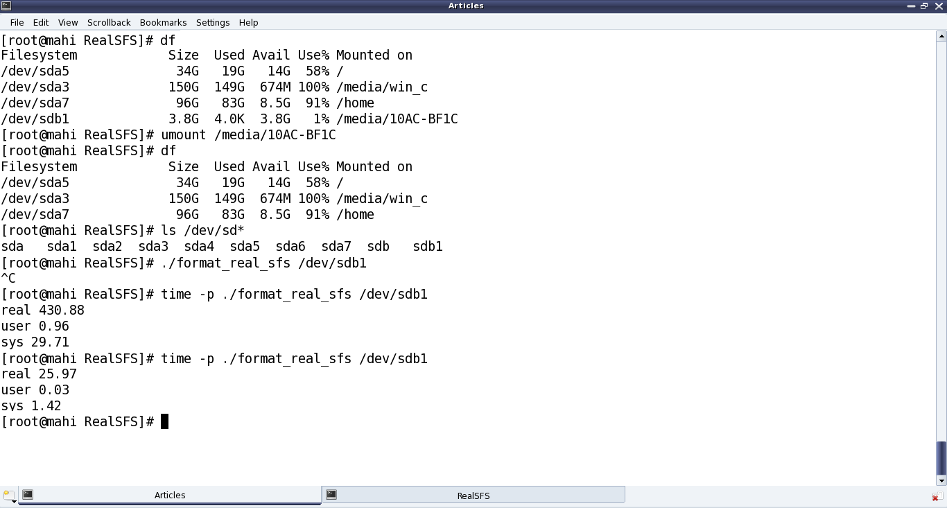
Using the previously formatted pen drive partition /dev/sdb1 or Re-formatting it using the format_real_sfs application: ./format_real_sfs /dev/sdb1. Caution: Please check out the complete detailed steps on this from the previous article, before you actually format it
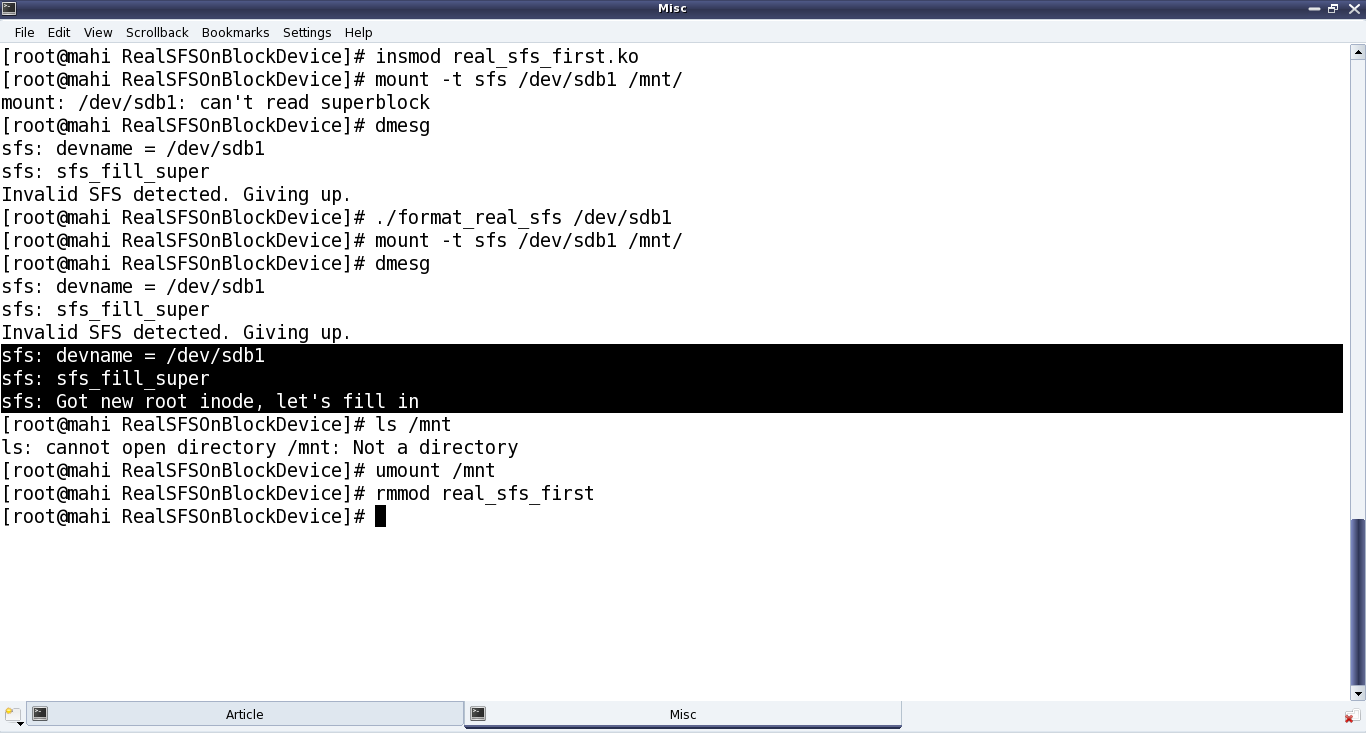
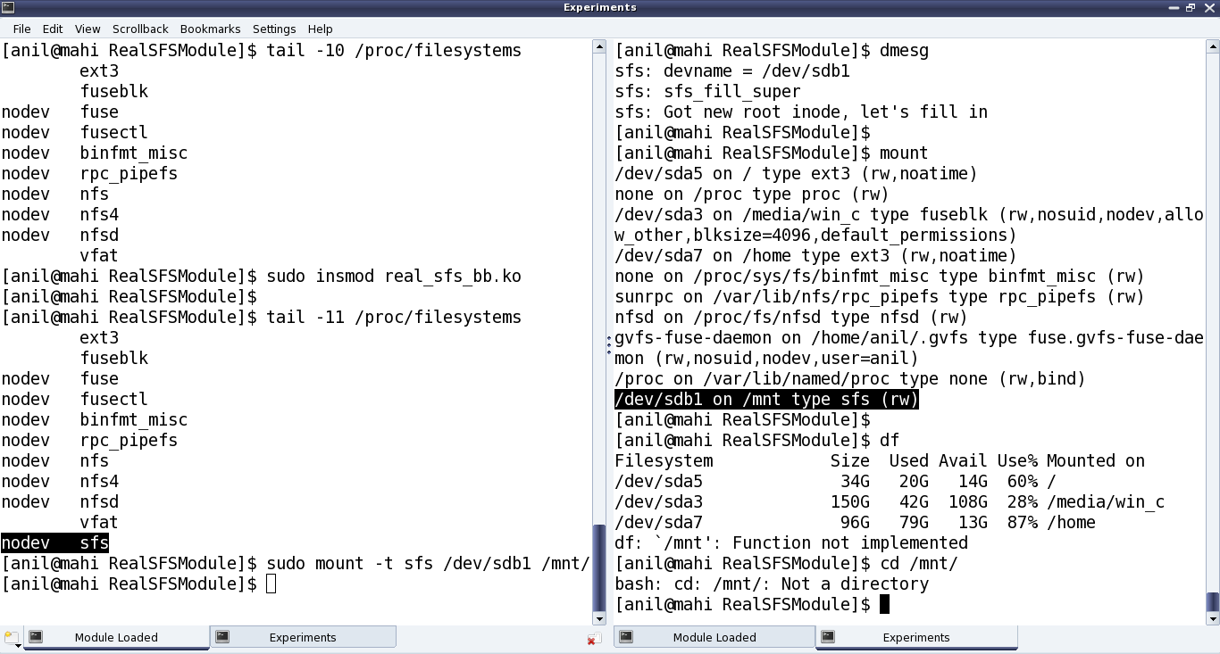
Mount the real SFS formatted partition: mount -t real_sfs /dev/sdb1 /mnt
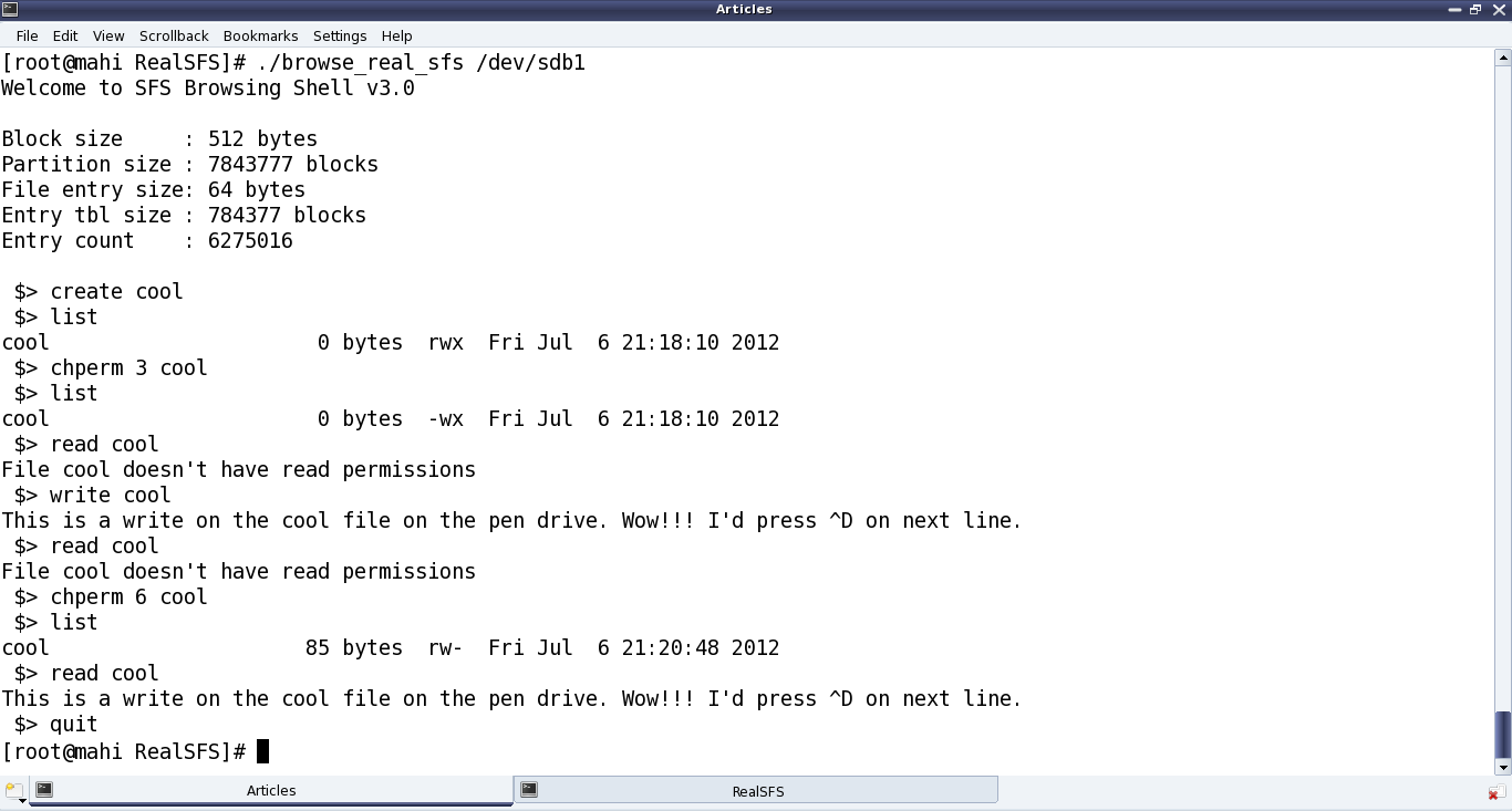
And … And what? Browse the mounting filesystem. Use your usual shell commands to operate on the file system: ls, cd, touch, vi, rm, chmod, …

Figure 40 shows the real SIMULA file system in action

Figure 40: The real SIMULA file system module in action

Realities behind the action

And if you really want to know, what are the additional enhancements Pugs added to the previous article’s code to get to this level, it is basically the following core system calls as part of the remaining 4 out of 5 set of structures of function pointers (in real_sfs.c):

write_inode (under struct super_operations) – sfs_write_inode() basically gets a pointer to an inode in the VFS’ inode cache, and is expected to sync that with the inode in physical hardware space file system. That is achieved by calling the appropriately modified sfs_update() (defined in real_sfs_ops.c) (adapted from the earlier browse_real_sfs application). The key parameter changes being passing the inode number instead of the filename and the actual timestamp instead of the flag for its update status. And accordingly, the call to filename based sfs_lookup() is being replaced by inode number based sfs_get_file_entry() (defined in real_sfs_ops.c), and additionally now the data blocks are also being freed (using sfs_put_data_block() (defined in real_sfs_ops.c)), if the file size has reduced. Note that sfs_put_data_block() (defined in real_sfs_ops.c) is a transformation of the put_data_block() from the browse_real_sfs application. Also, note the interesting mapping to / from the VFS inode number from / to our zero-based file entry indices, using the macros S2V_INODE_NUM() / V2S_INODE_NUM() in real_sfs_ops.h.
And finally, underlying write is being achieved using write_to_real_sfs(), a function added in real_sfs_ops.c, very similar to read_from_real_sfs() (already there in real_sfs_ops.c), except the direction reversal of the data transfer and marking the buffer dirty to be synced up with the physical content. Alongwith, in real_sfs_ops.c, two wrapper functions read_entry_from_real_sfs() (using read_from_real_sfs()) and write_entry_to_real_sfs() (using write_to_real_sfs()) have been written and used respectively for the specific requirements of reading and writing the file entries, to increase the code readability. sfs_write_inode() and sfs_update() are shown in the code snippet below. sfs_write_inode() has been written in the file real_sfs.c. For others, check out the file real_sfs_ops.c

#if (LINUX_VERSION_CODE < KERNEL_VERSION(2,6,34))
static int sfs_write_inode(struct inode *inode, int do_sync)
#else
static int sfs_write_inode(struct inode *inode, struct writeback_control *wbc)
#endif
{
	sfs_info_t *info = (sfs_info_t *)(inode->i_sb->s_fs_info);
	int size, timestamp, perms;

	printk(KERN_INFO "sfs: sfs_write_inode (i_ino = %ld)\n", inode->i_ino);

	if (!(S_ISREG(inode->i_mode))) // Real SFS deals only with regular files
		return 0;

	size = i_size_read(inode);
	timestamp = inode->i_mtime.tv_sec > inode->i_ctime.tv_sec ?
			inode->i_mtime.tv_sec : inode->i_ctime.tv_sec;
	perms = 0;
	perms |= (inode->i_mode & (S_IRUSR | S_IRGRP | S_IROTH)) ? 4 : 0;
	perms |= (inode->i_mode & (S_IWUSR | S_IWGRP | S_IWOTH)) ? 2 : 0;
	perms |= (inode->i_mode & (S_IXUSR | S_IXGRP | S_IXOTH)) ? 1 : 0;

	printk(KERN_INFO "sfs: sfs_write_inode with %d bytes @ %d secs w/ %o\n",
		size, timestamp, perms);

	return sfs_update(info, inode->i_ino, &size, &timestamp, &perms);
}

int sfs_update(sfs_info_t *info, int vfs_ino, int *size, int *timestamp, int *perms)
{
	sfs_file_entry_t fe; 
	int i;
	int retval;

	if ((retval = sfs_get_file_entry(info, vfs_ino, &fe)) < 0) 
	{   
		return retval; 
	}   
	if (size) fe.size = *size;
	if (timestamp) fe.timestamp = *timestamp;
	if (perms && (*perms <= 07)) fe.perms = *perms;

	for (i = (fe.size + info->sb.block_size - 1) / info->sb.block_size;
		i < SIMULA_FS_DATA_BLOCK_CNT; i++)
	{   
		if (fe.blocks[i])
		{   
			sfs_put_data_block(info, fe.blocks[i]);
			fe.blocks[i] = 0;
		}   
	}   

	return write_entry_to_real_sfs(info, V2S_INODE_NUM(vfs_ino), &fe);
}

create, unlink, lookup (under struct inode_operations) – All the 3 functions sfs_inode_create(), sfs_inode_unlink(), sfs_inode_lookup() have the 2 common parameters (the parent’s inode pointer and the pointer to the directory entry for the file in consideration), and these respectively create, delete, and lookup an inode corresponding to their directory entry pointed by their parameter, say dentry.
sfs_inode_lookup() basically searches for the existence of the filename underneath using the appropriately modified sfs_lookup() (defined in real_sfs_ops.c) (adapted from the earlier browse_real_sfs application – the adoption being replacing the user space lseek()+read() combo by the read_entry_from_real_sfs()). If filename is not found, then it invokes the generic kernel function d_splice_alias() to create a new inode entry in the underlying file system, for the same, and then attaches it to the directory entry pointed by dentry. Otherwise, it just attaches the inode from VFS’ inode cache (using generic kernel function d_add()). This inode, if obtained fresh (I_NEW), needs to be filled in with the real SFS looked up file attributes. In all the above implementations and in those to come, a few basic assumptions have been made, namely:
- Real SFS maintains mode only for user and that is mapped to all 3 of user, group, other of the VFS inode
- Real SFS maintains only one timestamp and that is mapped to all 3 of created, modified, accessed times of the VFS inode.
sfs_inode_create() and sfs_inode_unlink() correspondingly invokes the transformed sfs_create() and sfs_remove() (defined in real_sfs_ops.c) (adapted from the earlier browse_real_sfs application), for respectively creating and clearing the inode entries at the underlying hardware space file system, apart from the usual inode cache operations, using new_inode()+insert_inode_locked(), d_instantiate() & inode_dec_link_count(), instead of the earlier learnt iget_locked(), d_add(). Apart from the permissions and file entry parameters, and replacing lseek()+read() combo by read_entry_from_real_sfs(), sfs_create() has an interesting transformation from user space to kernel space: time(NULL) to get_seconds(). And in both of sfs_create() and sfs_remove() the user space lseek()+write() combo has been replaced by the obvious write_entry_to_real_sfs(). Check out all the above mentioned code pieces in the files real_sfs.c and real_sfs_ops.c, as mentioned.
readpage, write_begin, writepage, write_end (under struct address_space_operations) – All these address space operations are basically to read and write blocks on the underlying filesystem, and are achieved using the respective generic kernel functions mpage_readpage(), block_write_begin(), block_write_full_page(), generic_write_end(). First one is prototyped in <linux/mpage.h> and remaining 3 in <linux/buffer_head.h>. Now, though these functions are generic enough, a little thought would show that the first three of these would ultimately have to do a real SFS specific transaction with the underlying block device (the hardware partition), using the corresponding block layer APIs. And that exactly is achieved by the real SFS specific function sfs_get_block(), which is being passed into and used by the first three functions, mentioned above.
sfs_get_block() (defined in real_sfs.c) is invoked to read a particular block number (iblock) of a file (denoted by an inode), into a buffer head (bh_result), optionally fetching (allocating) a new block. So for that, the block array of corresponding real SFS inode is looked up into and then the corresponding block of the physical partition is fetched using the kernel API map_bh(). Again note that to fetch a new block, we invoke the sfs_get_data_block() (defined in real_sfs_ops.c), which is again a transformation of the get_data_block() from the browse_real_sfs application. Also, in case of a new block allocation, the real SFS inode is also updated underneath, using sfs_update_file_entry() – a one liner implementation in real_sfs_ops.c. Code snippet below shows the sfs_get_block() implementation.

static int sfs_get_block(struct inode *inode, sector_t iblock,
				struct buffer_head *bh_result, int create)
{
	struct super_block *sb = inode->i_sb;
	sfs_info_t *info = (sfs_info_t *)(sb->s_fs_info);
	sfs_file_entry_t fe;
	sector_t phys;
	int retval;

	printk(KERN_INFO "sfs: sfs_get_block called for I: %ld, B: %llu, C: %d\n",
		inode->i_ino, (unsigned long long)(iblock), create);

	if (iblock >= SIMULA_FS_DATA_BLOCK_CNT)
	{
		return -ENOSPC;
	}
	if ((retval = sfs_get_file_entry(info, inode->i_ino, &fe)) < 0)
	{
		return retval;
	}
	if (!fe.blocks[iblock])
	{
		if (!create)
		{
			return -EIO;
		}
		else
		{
			if ((fe.blocks[iblock] = sfs_get_data_block(info)) ==
				INV_BLOCK)
			{
				return -ENOSPC;
			}
			if ((retval = sfs_update_file_entry(info, inode->i_ino, &fe))
				< 0) 
			{   
				return retval;
			}
		}
	}
	phys = fe.blocks[iblock];
	map_bh(bh_result, sb, phys);

	return 0;
}

open, release, read, write, aio_read/read_iter (since kernel v3.16), aio_write/write_iter (since kernel v3.16), fsync (under a regular file’s struct file_operations) – All these operations should basically go through the buffer cache, i.e. should be implemented using the address space operations. And this being a common requirement, the kernel provides a generic set of kernel APIs, namely generic_file_open(), do_sync_read()/new_sync_read() (since kernel v3.16), do_sync_write()/new_sync_write() (since kernel v3.16), generic_file_aio_read()/generic_file_read_iter() (since kernel v3.16), generic_file_aio_write()/generic_file_write_iter() (since kernel v3.16), simple_sync_file()/noop_fsync() (since kernel v2.6.35). Moreover, the address space operations read & write are no longer required to be given since kernel v4.1. Note that there is no API for release, as it is a ‘return 0‘ API. Check out the real_sfs.c file for the exact definition of struct file_operations sfs_fops.
readdir/iterate (since kernel v3.11) (under a directory’s struct file_operations) – sfs_readdir()/sfs_iterate() primarily reads the directory entries of an underlying directory (denoted by file), and fills it up into the VFS directory entry cache (pointed by dirent parameter) using the parameter function filldir, or into the directory context (pointed by ctx parameter) (since kernel v3.11).
As real SFS has only one directory, the top one, this function basically fills up the directory entry cache with directory entries for all the files in the underlying file system, using the transformed sfs_list() (defined in real_sfs_ops.c), adapted from the browse_real_sfs application. Check out the real_sfs.c file for the complete sfs_readdir()/sfs_iterate() implementation, which starts with filling directory entries for ‘.‘ (current directory) and ‘..‘ (parent directory) using parameter function filldir(), or generic kernel function dir_emit_dots() (since kernel v3.11), and then for all the files of the real SFS, using sfs_list().
put_super (under struct super_operations) – The previous custom implementation sfs_kill_sb() (pointed by kill_sb) has been enhanced by separating it into the custom part being put into sfs_put_super() (and now pointed by put_super), and the standard kill_block_super() being directly pointed by kill_sb. Check out the file real_sfs.c for all these changes.

With all these in place, one could see the amazing demo by Pugs in action, as shown in Figure 40. And don’t forget watching the live log in /var/log/messages using a ‘tail -f /var/log/messages‘, matching it with every command you issue on the mounted real SFS file system. This would give you the best insight into when does which system call gets called. Or, in other words which application invokes which system call from the file system front. For tracing all the system calls invoked by an application/command, use strace with the command, e.g. type ‘strace ls‘ instead of just ‘ls‘.

Notes

On distros like Ubuntu, you may find the log under /var/log/syslog instead of /var/log/messages

Playing with Graphs

1 Reply

This twenty-fourth article of the mathematical journey through open source, demonstrates the concepts of graph theory for playing with graphs using the graphs package of Maxima.

<< Twenty-third Article

In our previous article, we familiarized ourselves with the notion of simple graphs, and how graphs package of Maxima allows us to create and visualize them. Assuming that knowledge, in this article, we are going to play with graphs and their properties, using the functionalities provided by Maxima’s graphs package.

Graph modifications

We have already created various graphs with create_graph() and make_graph() functions of the graphs package of Maxima. What if we want to modify some existing graphs, say by adding or removing some edges or vertices? Exactly for such operations, Maxima provides the following functions:

add_edge(<edge>, <g>) – Adds <edge> into the graph <g>
add_edges(<edge_list>, <g>) – Adds edges specified by <edge_list> into the graph <g>
add_vertex(<vertex>, <g>) – Adds <vertex> into the graph <g>
add_vertices(<vertex_list>, <g>) – Adds vertices specified by <vertex_list> into the graph <g>
connect_vertices(<u_list>, <v_list>, <g>) – Connects all vertices from <u_list> to all vertices in <v_list> in the graph <g>
contract_edge(<edge>, <g>) – Merges the vertices of the <edge> and the edges incident on those vertices, in the graph <g>
remove_edge(<edge>, <g>) – Removes the <edge> from the graph <g>
remove_vertex(<vertex>, <g>) – Removes the <vertex> and the associated edges from the graph <g>

Some of the above functions are demonstrated below:

$ maxima -q
(%i1) load(graphs)$ /* Loading the graphs package */
...
0 errors, 0 warnings
(%i2) g: create_graph(4, [[0, 1], [0, 2]]);
(%o2)                     GRAPH(4 vertices, 2 edges)
(%i3) print_graph(g)$

Graph on 4 vertices with 2 edges.
Adjacencies:
  3 :
  2 :  0
  1 :  0
  0 :  2  1
(%i4) add_edge([1, 2], g)$
(%i5) print_graph(g)$

Graph on 4 vertices with 3 edges.
Adjacencies:
  3 :
  2 :  1  0
  1 :  2  0
  0 :  2  1
(%i6) contract_edge([0, 1], g)$
(%i7) print_graph(g)$

Graph on 3 vertices with 1 edges.
Adjacencies:
  3 :
  2 :  0
  0 :  2

In the above examples, if we do not intend to modify the original graph, we may make a copy of it using copy_graph(), and then operate on the copy, as follows:

(%i8) h: copy_graph(g);
(%o8)                     GRAPH(3 vertices, 1 edges)
(%i9) add_vertex(1, h)$
(%i10) print_graph(h)$

Graph on 4 vertices with 1 edges.
Adjacencies:
  1 :
  0 :  2
  2 :  0
  3 :
(%i11) print_graph(g)$ /* Notice g is unmodified */

Graph on 3 vertices with 1 edges.
Adjacencies:
  3 :
  2 :  0
  0 :  2
(%i12) quit();

Advanced graph creations

New graphs can also be created based on existing graphs and their properties by various interesting operations. Few of them are:

underlying_graph(<dg>) – Returns the underlying graph of the directed graph <dg>
complement_graph(<g>) – Returns the complement graph of graph <g>
line_graph(<g>) – Returns a graph that represents the adjacencies between the edges of graph <g>
graph_union(<g1>, <g2>) – Returns a graph with edges and vertices of both graphs <g1> and <g2>
graph_product(<g1>, <g2>) – Returns the Cartesian product of graphs <g1> and <g2>

Here are some examples to demonstrate the simpler functions:

$ maxima -q
(%i1) load(graphs)$
...
0 errors, 0 warnings
(%i2) g: create_graph(4, [[0, 1], [0, 2], [0, 3]], directed = true);
(%o2)                     DIGRAPH(4 vertices, 3 arcs)
(%i3) print_graph(g)$

Digraph on 4 vertices with 3 arcs.
Adjacencies:
  3 :
  2 :
  1 :
  0 :  3  2  1
(%i4) h: underlying_graph(g);
(%o4)                     GRAPH(4 vertices, 3 edges)
(%i5) print_graph(h)$

Graph on 4 vertices with 3 edges.
Adjacencies:
  0 :  1  2  3
  1 :  0
  2 :  0
  3 :  0
(%i6) print_graph(complement_graph(h))$

Graph on 4 vertices with 3 edges.
Adjacencies:
  3 :  2  1
  2 :  3  1
  1 :  3  2
  0 :
(%i7) print_graph(graph_union(h, complement_graph(h)))$

Graph on 8 vertices with 6 edges.
Adjacencies:
  4 :
  5 :  6  7
  6 :  5  7
  7 :  5  6
  3 :  0
  2 :  0
  1 :  0
  0 :  3  2  1
(%i8) quit();

Basic graph properties

graph_order(<g>), vertices(<g>) returns the number of vertices and the list of vertices, respectively, in the graph <g>. graph_size(<g>), edges(<g>) returns the number of edges and the list of edges, respectively, in the graph <g>.

A graph is a collection of vertices and edges. Hence, most of its properties are centred around them. The following are graph related predicates provided by the graphs package of Maxima:

is_graph(<g>) – returns true if <g> is a graph, false otherwise
is_digraph(<g>) – returns true if <g> is a directed graph, false otherwise
is_graph_or_digraph(<g>) – returns true if <g> is a graph or a directed graph, false otherwise
is_connected(<g>) – returns true if graph <g> is connected, false otherwise
is_planar(<g>) – returns true if graph <g> can be placed on a plane without its edges crossing over each other, false otherwise
is_tree(<g>) – returns true if graph <g> has no simple cycles, false otherwise
is_biconnected(<g>) – returns true if graph <g> will remain connected even after removal of any one its vertices and the edges incident on that vertex, false otherwise
is_bipartite(<g>) – returns true if graph <g> is bipartite, i.e. 2-colourable, false otherwise
is_isomorphic(<g1>, <g2>) – returns true if graphs <g1> and <g2> have the same number of vertices and are connected in the same way, false otherwise. And, isomorphism(<g1>, <g2>) returns an isomorphism (that is a one-to-one onto mapping) between the graphs <g1> and <g2>, if it exists.
is_edge_in_graph(<edge>, <g>) – returns true if <edge> is in graph <g>, false otherwise
is_vertex_in_graph(<vertex>, <g>) – returns true if <vertex> is in graph <g>, false otherwise

The following example specifically demonstrates the isomorphism property, from the list above:

$ maxima -q
(%i1) load(graphs)$
...
0 errors, 0 warnings
(%i2) g1: create_graph(3, [[0, 1], [0, 2]]);
(%o2)                     GRAPH(3 vertices, 2 edges)
(%i3) g2: create_graph(3, [[1, 2], [0, 2]]);
(%o3)                     GRAPH(3 vertices, 2 edges)
(%i4) is_isomorphic(g1, g2);
(%o4)                                true
(%i5) isomorphism(g1, g2);
(%o5)                      [2 -> 0, 1 -> 1, 0 -> 2]
(%i6) quit();

Graph neighbourhoods

Lot of properties of graphs are to do with vertex and edge neighbourhoods, also referred as adjacencies.

For example, a graph itself could be represented by an adjacency list or matrix, which specifies the vertices adjacent to the various vertices in the graph. adjacency_matrix(<g>) returns the adjacency matrix of the graph <g>.

Number of edges incident on a vertex is called the valency or degree of the vertex, and could be obtained using vertex_degree(<v>, <g>). degree_sequence(<g>) returns the list of degrees of all the vertices of the graph <g>. In case of a directed graph, the degrees could be segregated as in-degree and out-degree, as per the edges incident into and out of the vertex, respectively. vertex_in_degree(<v>, <dg>) and vertex_out_degree(<v>, <dg>) respectively return the in-degree and out-degree for the vertex <v> of the directed graph <dg>.

neighbors(<v>, <g>), in_neighbors(<v>, <dg>), out_neighbors(<v>, <dg>) respectively return the list of adjacent vertices, adjacent in-vertices, adjacent out-vertices of the vertex <v> in the corresponding graphs.

average_degree(<g>) computes the average of degrees of all the vertices of the graph <g>. max_degree(<g>) finds the maximal degree of vertices of the graph <g>, and returns one such vertex alongwith. min_degree(<g>) finds the minimal degree of vertices of the graph <g>, and returns one such vertex alongwith.

Here follows a neighbourhood related demonstration:

$ maxima -q
(%i1) load(graphs)$
...
0 errors, 0 warnings
(%i2) g: create_graph(4, [[0, 1], [0, 2], [0, 3], [1, 2]]);
(%o2)                     GRAPH(4 vertices, 4 edges)
(%i3) string(adjacency_matrix(g)); /* string for output in single line */
(%o3)           matrix([0,0,0,1],[0,0,1,1],[0,1,0,1],[1,1,1,0])
(%i4) degree_sequence(g);
(%o4)                            [1, 2, 2, 3]
(%i5) average_degree(g);
(%o5)                                  2
(%i6) neighbors(0, g);
(%o6)                              [3, 2, 1]
(%i7) quit();

Graph connectivity

A graph is ultimately about connections, and hence lots of graph properties are centred around connectivity.

vertex_connectivity(<g>) returns the minimum number of vertices that need to be removed from the graph <g> to make the graph <g> disconnected. Similarly, edge_connectivity(<g>) returns the minimum number of edges that need to be removed from the graph <g> to make the graph <g> disconnected.

vertex_distance(<u>, <v>, <g>) returns the length of the shortest path between the vertices <u> and <v> in the graph <g>. The actual path could be obtained using shortest_path(<u>, <v>, <g>).

girth(<g>) returns the length of the shortest cycle in graph <g>.

vertex_eccentricity(<v>, <g>) returns the maximum of the vertex distances of vertex <v> with any other vertex in the connected graph <g>.

diameter(<g>) returns the maximum of the vertex eccentricities of all the vertices in the connected graph <g>.

radius(<g>) returns the minimum of the vertex eccentricities of all the vertices in the connected graph <g>.

graph_center(<g>) returns the list of vertices that have eccentricities equal to the radius of the connected graph <g>.

graph_periphery(<g>) is the list of vertices that have eccentricities equal to the diameter of the connected graph.

A minimal connectivity related demonstration for the graph shown in Figure 29 follows:

$ maxima -q
(%i1) load(graphs)$
...
0 errors, 0 warnings
(%i2) g: create_graph(9, [[0, 1], [0, 2], [1, 8], [8, 3], [2, 3], [3, 4], [4, 5],
        [3, 6], [3, 7]]);
(%o2)                     GRAPH(9 vertices, 9 edges)
(%i3) vertex_connectivity(g);
(%o3)                                  1
(%i4) edge_connectivity(g);
(%o4)                                 1
(%i5) shortest_path(0, 7, g);
(%o5)                           [0, 2, 3, 7]
(%i6) vertex_distance(0, 7, g);
(%o6)                                 3
(%i7) girth(g);
(%o7)                                 5
(%i8) diameter(g);
(%o8)                                 4
(%i9) radius(g);
(%o9)                                 2
(%i10) graph_center(g);
(%o10)                                [3]
(%i11) graph_periphery(g);
(%o11)                             [5, 1, 0]

Figure 29: Graph connectivities

Vertex 3 is the only centre of the graph and 0, 1, 5 are the peripheral vertices of the graph.

Graph colouring

Graph colouring has been a fascinating topic in graph theory, since its inception. It is all about colouring the vertices or edges of a graph in such a way that no adjacent elements (vertex or edge) have the same colour.

Smallest number of colours needed to colour the vertices of a graph, such that no two adjacent vertices have the same colour, is called the chromatic number of the graph. chromatic_number(<g>) computes the same. vertex_coloring(<g>) returns a list representing the colouring of the vertices of <g>, along with the chromatic number.

Smallest number of colours needed to colour the edges of a graph, such that no two adjacent edges have the same colour, is called the chromatic index of the graph. chromatic_index(<g>) computes the same. edge_coloring(<g>) returns a list representing the colouring of the edges of <g>, along with the chromatic index.

The following demonstration continues colouring the graph from the above demonstration:

(%i12) chromatic_number(g);
(%o12)                                 3
(%i13) vc: vertex_coloring(g);
(%o13) [3, [[0, 3], [1, 1], [2, 2], [3, 1], [4, 2], [5, 1], [6, 2], [7, 2], [8, 2]]]
(%i14) chromatic_index(g);
(%o14)                                 5
(%i15) ec: edge_coloring(g);
(%o15) [5, [[[0, 1], 1], [[0, 2], 2], [[1, 8], 2], [[3, 8], 5], [[2, 3], 1], 
                           [[3, 4], 2], [[4, 5], 1], [[3, 6], 3], [[3, 7], 4]]]
(%i16) draw_graph(g, vertex_coloring=vc, edge_coloring=ec, vertex_size=5,
        edge_width=3, show_id=true)$
(%i17) quit();

Figure 30 shows the coloured version of the graph, as obtained by %i16.

Figure 30: Graph colouring

Bon voyage

With this article, we have completed a 2 year long mathematical journey through open source, starting from mathematics in Shell, covering Bench Calculator, Octave, and finally concluding with Maxima. I take this opportunity to thank my readers and wish them bon voyage with whatever they have gained through our interactions. However, this is not the end – get set for our next odyssey.

The Semester Project – Part VI: File System on Block Device

1 Reply

This twenty-third article, which is part of the series on Linux device drivers, enhances the previously written bare bone file system module, to connect with a real hardware partition.

<< Twenty-second Article

Since the last bare bone file system, the first thing which Pugs figured out was how to read from the underlying block device. Following is a typical way of doing it:

struct buffer_head *bh;

bh = sb_bread(sb, block); /* sb is the struct super_block pointer */
// bh->b_data contains the data
// Once done, bh should be released using:
brelse(bh);

To do the above and various other real SFS (Simula File System) operations, Pugs’ felt a need to have his own handle to be a key parameter, which he added as follows (in previous real_sfs_ds.h):

typedef struct sfs_info
{
	struct super_block *vfs_sb; /* Super block structure from VFS for this fs */
	sfs_super_block_t sb; /* Our fs super block */
	byte1_t *used_blocks; /* Used blocks tracker */
} sfs_info_t;

The main idea behind this was to put all required static global variables in a single structure, and point that by the private data pointer of the file system, which is s_fs_info pointer in the struct super_block structure. With that, the key changes in the fill_super_block() (in previous real_sfs_bb.c file) becomes:

Allocate the structure for the handle, using kzalloc()
Initialize the structure for the handle (through init_browsing())
Read the physical super block, verify and translate info from it into the VFS super block (through init_browsing())
Point it by s_fs_info (through init_browsing())
Update the VFS super block, accordingly

Accordingly, the error handling code would need to do the shut_browsing(info) and kfree(info). And, that would additionally also need to go along with the function corresponding to the kill_sb function pointer, defined in the previous real_sfs_bb.c by kill_block_super, called during umount.

Here’s the various code pieces:

#include <linux/slab.h> /* For kzalloc, ... */
...
static int sfs_fill_super(struct super_block *sb, void *data, int silent)
{
	sfs_info_t *info;

	if (!(info = (sfs_info_t *)(kzalloc(sizeof(sfs_info_t), GFP_KERNEL))))
		return -ENOMEM;
	info->vfs_sb = sb;
	if (init_browsing(info) < 0)
	{
		kfree(info);
		return -EIO;
	}
	/* Updating the VFS super_block */
	sb->s_magic = info->sb.type;
	sb->s_blocksize = info->sb.block_size;
	sb->s_blocksize_bits = get_bit_pos(info->sb.block_size);

	...
}

static void sfs_kill_sb(struct super_block *sb)
{
	sfs_info_t *info = (sfs_info_t *)(sb->s_fs_info);

	kill_block_super(sb);
	if (info)
	{
		shut_browsing(info);
		kfree(info);
	}
}

kzalloc() in contrast to kmalloc(), also zeroes out the allocated location. get_bit_pos() is a simple Pugs’ way to compute logarithm base 2, as follows:

static int get_bit_pos(unsigned int val)
{
	int i;

	for (i = 0; val; i++)
	{
		val >>= 1;
	}
	return (i - 1);
}

And init_browsing(), shut_browsing() are basically the transformations of the earlier user-space functions of browse_real_sfs.c into kernel-space code real_sfs_ops.c, prototyped in real_sfs_ops.h. This basically involves the following transformations:

“int sfs_handle” into “sfs_info_t *info“
lseek() & read() into the read from the block device using sb_bread()
calloc() into vmalloc() & then appropriate initialization by zeros.
free() into vfree()

Here’s the transformed init_browsing() and shut_browsing() in real_sfs_ops.c:

#include <linux/fs.h> /* For struct super_block */
#include <linux/errno.h> /* For error codes */
#include <linux/vmalloc.h> /* For vmalloc, ... */

#include "real_sfs_ds.h"
#include "real_sfs_ops.h"

int init_browsing(sfs_info_t *info)
{
	byte1_t *used_blocks;
	int i, j;
	sfs_file_entry_t fe;
	int retval;

	if ((retval = read_sb_from_real_sfs(info, &info->sb)) < 0)
	{
		return retval;
	}
	if (info->sb.type != SIMULA_FS_TYPE)
	{
		printk(KERN_ERR "Invalid SFS detected. Giving up.\n");
		return -EINVAL;
	}

	/* Mark used blocks */
	used_blocks = (byte1_t *)(vmalloc(info->sb.partition_size));
	if (!used_blocks)
	{
		return -ENOMEM;
	}
	for (i = 0; i < info->sb.data_block_start; i++)
	{
		used_blocks[i] = 1;
	}
	for (; i < info->sb.partition_size; i++)
	{
		used_blocks[i] = 0;
	}

	for (i = 0; i < info->sb.entry_count; i++)
	{
		if ((retval = read_from_real_sfs(info,
					info->sb.entry_table_block_start,
					i * sizeof(sfs_file_entry_t),
					&fe, sizeof(sfs_file_entry_t))) < 0)
		{
			vfree(used_blocks);
			return retval;
		}
		if (!fe.name[0]) continue;
		for (j = 0; j < SIMULA_FS_DATA_BLOCK_CNT; j++)
		{
			if (fe.blocks[j] == 0) break;
			used_blocks[fe.blocks[j]] = 1;
		}
	}

	info->used_blocks = used_blocks;
	info->vfs_sb->s_fs_info = info;
	return 0;
}
void shut_browsing(sfs_info_t *info)
{
	if (info->used_blocks)
		vfree(info->used_blocks);
}

Similarly, all other functions in browse_real_sfs.c would also have to be transformed, one by one. Also, note the read from the underlying block device is being captured by the two functions, namely read_sb_from_real_sfs() and read_from_real_sfs(), which are coded as follows:

#include <linux/buffer_head.h> /* struct buffer_head, sb_bread, ... */
#include <linux/string.h> /* For memcpy */

#include "real_sfs_ds.h"

static int read_sb_from_real_sfs(sfs_info_t *info, sfs_super_block_t *sb)
{
	struct buffer_head *bh;

	if (!(bh = sb_bread(info->vfs_sb, 0 /* Super block is the 0th block */)))
	{
		return -EIO;
	}
	memcpy(sb, bh->b_data, SIMULA_FS_BLOCK_SIZE);
	brelse(bh);
	return 0;
}
static int read_from_real_sfs(sfs_info_t *info, byte4_t block,
				byte4_t offset, void *buf, byte4_t len)
{
	byte4_t block_size = info->sb.block_size;
	byte4_t bd_block_size = info->vfs_sb->s_bdev->bd_block_size;
	byte4_t abs;
	struct buffer_head *bh;

	/*
	 * Translating the real SFS block numbering to underlying block device
	 * block numbering, for sb_bread()
	 */
	abs = block * block_size + offset;
	block = abs / bd_block_size;
	offset = abs % bd_block_size;
	if (offset + len > bd_block_size) // Should never happen
	{
		return -EINVAL;
	}
	if (!(bh = sb_bread(info->vfs_sb, block)))
	{
		return -EIO;
	}
	memcpy(buf, bh->b_data + offset, len);
	brelse(bh);
	return 0;
}

All the above code pieces put in together as the real_sfs_minimal.c (based on the file real_sfs_bb.c created earlier), real_sfs_ops.c, real_sfs_ds.h (based on the same file created earlier), real_sfs_ops.h, and a supporting Makefile, along with the previously created format_real_sfs.c application are available from rsfs_on_block_device_code.tbz2.

Real SFS on block device

Once compiled using make, getting the real_sfs_first.ko driver, Pugs didn’t expect it to be way different from the previous real_sfs_bb.ko driver, but at least now it should be reading and verifying the underlying partition. And for that he first tried mounting the usual partition of a pen drive to get an “Invalid SFS detected” message in dmesg output; and then after formatting it. Note the same error of “Not a directory”, etc as in previous article, still existing – as anyways it is still very similar to the previous bare bone driver – the core functionalities yet to be implemented – just that it is now on a real block device partition. Figure 39 shows the exact commands for all these steps.

Figure 39: Connecting the SFS module with the pen drive partition

Note: “./format_real_sfs” and “mount” commands may take lot of time (may be in minutes), depending on the partition size. So, preferably use a partition, say less than 1MB.

With this important step of getting the file system module interacting with the underlying block device, the last step for Pugs would be to do the other transformations from browse_real_sfs.c and accordingly use them in the SFS module.

Twenty-fourth Article >>

Visualizing Graph Theory

2 Replies

This twenty-third article of the mathematical journey through open source, introduces graph theory with visuals using the graphs package of Maxima.

<< Twenty-second Article

Graphs here refer to the structures formed using some points (or vertices), and some lines (or edges) connecting them. A simple example would be a graph with two vertices, say ‘0’ & ‘1’, and an edge between ‘0’ and ‘1’. If all the edges of a graph have a sense of direction from one vertex to another, typically represented by an arrow at their end(s), we call that a directed graph with directed edges. In such a case, we consider the edges to be not between two vertices but from one vertex to another vertex. Directed edges are also referred to as arcs. In the above example, we could have two directed arcs, one from ‘0’ to ‘1’, and another from ‘1’ to ‘0’. Figures 24 & 25 show an undirected and a directed graph, respectively.

Figure 24: Simple undirected graph

Figure 25: Simple directed graph

Graph creation & visualization

Now, how did we get those figures? Using the graphs package of Maxima, which is loaded by invoking load(graphs) at the Maxima prompt. In the package, vertices are represented by whole numbers 0, 1, … and an edge is represented as a list of its two vertices. Using these notations, we can create graphs using the create_graph(<vertex_list>, <edge_list>[, directed]) function. And, then draw_graph(<graph>[, <option1>, <option2>, …]) would draw the graph pictorially. Code snippet below shows the same in action:

$ maxima -q
(%i1) load(graphs)$
...
0 errors, 0 warnings
(%i2) g: create_graph([0, 1], [[0, 1]])$
(%i3) dg: create_graph([0, 1], [[0, 1]], directed=true)$
(%i4) draw_graph(g, show_id=true, vertex_size=5, vertex_color=yellow)$
(%i5) draw_graph(dg, show_id=true, vertex_size=5, vertex_color=yellow)$

The “show_id=true” option draws the vertex numbers, and vertex_size and vertex_color draws the vertices with the corresponding size and colour.

Note that a graph without any duplicate edges and without any loops is called a simple graph. And, an edge from a vertex U to V is not duplicate of an edge from vertex V to U in a directed graph but is duplicate in an undirected graph. Maxima’s package supports only simple graphs, i.e. graphs without duplicate edges and loops.

A simple graph can also be equivalently represented by adjacency of vertices, meaning by lists of adjacent vertices for every vertex. print_graph(<graph>) exactly displays those lists. The following code demonstration, in continuation from the previous code, demonstrates that:

(%i6) print_graph(g)$

Graph on 2 vertices with 1 edges.
Adjacencies:
  1 :  0
  0 :  1
(%i7) print_graph(dg)$

Digraph on 2 vertices with 1 arcs.
Adjacencies:
  1 :
  0 :  1
(%i8) quit();

create_graph(<num_of_vertices>, <edge_list>[, directed]) is another way of creating a graph using create_graph(). Here, the vertices are created as 0, 1, …, <num_of_vertices> – 1. So, both the above graphs could equivalently be created as follows:

$ maxima -q
(%i1) load(graphs)$
...
0 errors, 0 warnings
(%i2) g: create_graph(2, [[0, 1]]);
(%o2)                     GRAPH(2 vertices, 1 edges)
(%i3) dg: create_graph(2, [[0, 1]], directed=true);
(%o3)                     DIGRAPH(2 vertices, 1 arcs)
(%i4) quit();

make_graph(<vertices>, <predicate>[, directed]) is another interesting way of creating a graph, based on vertex connectivity conditions specified by the <predicate> function. <vertices> could be an integer or a set/list of vertices. If it is a positive integer, then the vertices would be 1, 2, …, <vertices>. In any case, <predicate> should be a function taking two arguments of the vertex type and returning true or false. make_graph() creates a graph with the vertices specified as above, and with the edges between the vertices for which the <predicate> function returns true.

A trivial case would be, if the <predicate> always returns true, then it would create a complete graph, i.e. a simple graph where all vertices are connected to each other. Here are a couple of demonstrations of make_graph():

$ maxima -q
(%i1) load(graphs)$
...
0 errors, 0 warnings
(%i2) f(i, j) := true$
(%i3) g: make_graph(6, f);
(%o3)                   GRAPH(6 vertices, 15 edges)
(%i4) draw_graph(g, show_id=true, vertex_color=yellow)$
(%i5) f(i, j) := is(mod(i, j)=0)$
(%i6) g: make_graph(10, f, directed = true);
(%o6)                  DIGRAPH(10 vertices, 17 arcs)
(%i7) draw_graph(g, show_id=true, vertex_color=yellow, vertex_size=4)$
(%i8) quit();

Figures 26 shows the output graphs from the above code.

Figure 26: More simple graphs

Graph varieties

One aware of graphs, would have known or at least heard of a variety of them. Here’s a list of some of them, available in Maxima’s graphs package (through functions):

Empty graph (empty_graph(n)) – Graph with a given n vertices but no edges
Complete graph (complete_graph(n)) – Simple graph with all possible edges for a given n vertices
Complete bipartite graph (complete_bipartite_graph(m, n)) – Simple graph with two set of vertices, having all possible edges between the vertices from the two sets, but with no edge between the vertices of the same set.
Cube graph (cube_graph(n)) – Graph representing an n-dimensional cube
Dodecahedron graph (dodecahedron_graph()) – Graph forming a 3-D polyhedron with 12 pentagonal faces
Cuboctahedron graph (cuboctahedron_graph()) – Graph forming a 3-D polyhedron with 8 triangular faces and 12 square faces
Icosahedron graph (icosahedron_graph()) – Graph forming a 3-D polyhedron with 20 triangular faces
Icosidodecahedron graph (icosidodecahedron_graph()) – Graph forming a 3-D uniform star polyhedron with 12 star faces and 20 triangular faces

And here follows a demonstration of the above, along with the visuals (left to right, top to bottom) in Figure 27:

$ maxima -q
(%i1) load(graphs)$
...
0 errors, 0 warnings
(%i2) g: empty_graph(5);
(%o2)                     GRAPH(5 vertices, 0 edges)
(%i3) draw_graph(g, show_id=true, vertex_color=yellow)$
(%i4) g: complete_graph(5);
(%o4)                     GRAPH(5 vertices, 10 edges)
(%i5) draw_graph(g, show_id=true, vertex_color=yellow)$
(%i6) g: complete_bipartite_graph(5, 3);
(%o6)                     GRAPH(8 vertices, 15 edges)
(%i7) draw_graph(g, show_id=true, vertex_color=yellow)$
(%i8) g: cube_graph(3);
(%o8)                    GRAPH(8 vertices, 12 edges)
(%i9) draw_graph(g, show_id=true, vertex_color=yellow)$
(%i10) g: cube_graph(4);
(%o10)                   GRAPH(16 vertices, 32 edges)
(%i11) draw_graph(g, show_id=true, vertex_color=yellow)$
(%i12) g: dodecahedron_graph();
(%o12)                   GRAPH(20 vertices, 30 edges)
(%i13) draw_graph(g, show_id=true, vertex_color=yellow)$
(%i14) g: cuboctahedron_graph();
(%o14)                   GRAPH(12 vertices, 24 edges)
(%i15) draw_graph(g, show_id=true, vertex_color=yellow)$
(%i16) g: icosahedron_graph();
(%o16)                   GRAPH(12 vertices, 30 edges)
(%i17) draw_graph(g, show_id=true, vertex_color=yellow)$
(%i18) g: icosidodecahedron_graph();
(%o18)                   GRAPH(30 vertices, 60 edges)
(%i19) draw_graph(g, show_id=true, vertex_color=yellow)$
(%i20) quit();

Figure 27: Graph varieties

Graph beauties

Graphs are really beautiful to visualize. Some of the many beautiful graphs, available in Maxima’s graphs package (through functions), are listed below:

Circulant graph (circulant_graph(n, [x, y, …])) – Graph with vertices 0, …, n-1, where every vertex is adjacent to its x^th, y^th, … vertices. Visually, it has a cyclic group of symmetries./li>
Flower graph (flower_snark(n)) – Graph like a flower with n petals and 4*n vertices
Wheel graph (wheel_graph(n)) – Graph like a wheel with n vertices
Clebsch graph (clebsch_graph()) – An another symmetrical graph beauty, named by J J Seidel
Frucht graph (frucht_graph()) – A graph with 12 vertices, 18 edges, and no nontrivial symmetries, such that every vertex have 3 neighbours. It is named after Robert Frucht
Grötzsch graph (grotzch_graph()) – A triangle-free graph with 11 vertices and 20 edges, named after Herbert Grötzsch
Heawood graph (heawood_graph()) – A symmetrical graph with 14 vertices and 21 edges, named after Percy John Heawood
Petersen graph (petersen_graph()) – A symmetrical graph with 10 vertices and 15 edges, named after Julius Petersen
Tutte graph (tutte_graph()) – A graph with 46 vertices and 69 edges, such that every vertex have 3 neighbours. It is named after W T Tutte

And here follows a demonstration of some of the above, along with the visuals (left to right, top to bottom) in Figure 28:

$ maxima -q
(%i1) load(graphs)$
...
0 errors, 0 warnings
(%i2) g: circulant_graph(10, [1, 3]);
(%o2)                   GRAPH(10 vertices, 20 edges)
(%i3) draw_graph(g, show_id=true, vertex_color=yellow)$
(%i4) g: circulant_graph(10, [1, 3, 4, 6]);
(%o4)                   GRAPH(10 vertices, 40 edges)
(%i5) draw_graph(g, show_id=true, vertex_color=yellow)$
(%i6) g: flower_snark(3);
(%o6)                   GRAPH(12 vertices, 18 edges)
(%i7) draw_graph(g, show_id=true, vertex_color=yellow)$
(%i8) g: flower_snark(5);
(%o8)                   GRAPH(20 vertices, 30 edges)
(%i9) draw_graph(g, show_id=true, vertex_color=yellow)$
(%i10) g: flower_snark(8);
(%o10)                   GRAPH(32 vertices, 48 edges)
(%i11) draw_graph(g, show_id=true, vertex_color=yellow)$
(%i12) g: flower_snark(10);
(%o12)                   GRAPH(40 vertices, 60 edges)
(%i13) draw_graph(g, show_id=true, vertex_color=yellow)$
(%i14) g: wheel_graph(3);
(%o14)                    GRAPH(4 vertices, 6 edges)
(%i15) draw_graph(g, show_id=true, vertex_color=yellow)$
(%i16) g: wheel_graph(4);
(%o16)                    GRAPH(5 vertices, 8 edges)
(%i17) draw_graph(g, show_id=true, vertex_color=yellow)$
(%i18) g: wheel_graph(5);
(%o18)                    GRAPH(6 vertices, 10 edges)
(%i19) draw_graph(g, show_id=true, vertex_color=yellow)$
(%i20) g: wheel_graph(10);
(%o20)                   GRAPH(11 vertices, 20 edges)
(%i21) draw_graph(g, show_id=true, vertex_color=yellow)$
(%i22) g: wheel_graph(100);
(%o22)                  GRAPH(101 vertices, 200 edges)
(%i23) draw_graph(g, show_id=true, vertex_color=yellow)$
(%i24) g: clebsch_graph();
(%o24)                   GRAPH(16 vertices, 40 edges)
(%i25) draw_graph(g, show_id=true, vertex_color=yellow)$
(%i26) g: grotzch_graph();
(%o26)                   GRAPH(11 vertices, 20 edges)
(%i27) draw_graph(g, show_id=true, vertex_color=yellow)$
(%i28) g: petersen_graph();
(%o28)                   GRAPH(10 vertices, 15 edges)
(%i29) draw_graph(g, show_id=true, vertex_color=yellow)$
(%i30) g: tutte_graph();
(%o30)                   GRAPH(46 vertices, 69 edges)
(%i31) draw_graph(g, show_id=true, vertex_color=yellow)$
(%i32) quit();

Figure 28: Graph beauties

What next?

With all these visualizations, you may be wondering, what to do with these apart from just staring at them. Visualizations were just to motivate you, visually. In fact, every graph has a particular set of properties, which distinguishes it from the other. And, there is a lot of beautiful mathematics involved with these properties. If you are motivated enough, watch out for playing around with these graphs and their properties.

Twenty-fourth Article >>

The Semester Project – Part V: File System Module Template

2 Replies

This twenty-second article, which is part of the series on Linux device drivers, lays out a bare bone file system module.

<< Twenty-first Article

With the formatting of the pen drive, the file system is all set in the hardware space. Now, it is the turn to decode that using a corresponding file system module in the kernel space, and accordingly provide the user space file system interface, for it to be browsed like any other file systems.

The 5 sets of System Calls

Unlike character or block drivers, the file system drivers involve not just one structure of function pointers, but instead 5 structures of function pointers, for the various interfaces, provided by a file system. These are:

struct file_system_type – contains functions to operate on the super block
struct super_operations – contains functions to operate on the inodes
struct inode_operations – contains functions to operate on the directory entries
struct file_operations – contains functions to operate on the file data (through page cache)
struct address_space_operations – contains page cache operations for the file data

With these, there were many new terms for Pugs. He referred the following glossary to understand the various terms used above and later in the file system module development:

Page cache or Buffer cache: Pool of RAM buffers, each of page size (typically 4096 bytes). These buffers are used as the cache for the file data read from the underlying hardware, thus increasing the performance of file operations
Inode: Structure containing the meta data / information of a file, like permissions, owner, etc. Though file name is a meta data of a file, for better space utilization, in typical Linux file systems, it is not kept in inode, instead in something called directory entries. Collection of inodes, is called an inode table
Directory entry: Structure containing the name and inode number of a file or directory. In typical Linux based file systems, a collection of directory entries for the immediate files and directories of say directory D, is stored in the data blocks of the directory D
Super block: Structure containing the information about the various data structures of the file systems, like the inode tables, … Basically the meta meta data, i.e. meta data for the meta data
Virtual File System (VFS): Conceptual file system layer interfacing the kernel space to user space in an abstract manner, showing “everything” as a file, and translating their operations from user to the appropriate entity in the kernel space

Each one of the above five structures contains a list of function pointers, which needs to be populated depending on what all features are there or to be supported in the file system (module). For example, struct file_system_type may contain system calls for mounting and unmounting a file system, basically operating on its super block; struct super_operations may contain inode read/write system calls; struct inode_operations may contain function to lookup directory entries; struct file_operations may generically operate on the page cached file data, which may in turn invoke page cache operations, defined in the struct address_space_operations. For these various operations, most of these functions will then interface with the corresponding underlying block device driver to ultimately operate with the formatted file system in the hardware space.

To start with Pugs laid out the complete framework of his real SFS module, but with minimal functionality, good enough to compile, load, and not crash the kernel. He populated only the first of these five structures – the struct file_system_type; and left all the others empty. Here’s the exact code of the structure definitions:

#include <linux/fs.h> /* For system calls, structures, ... */

static struct file_system_type sfs;
static struct super_operations sfs_sops;
static struct inode_operations sfs_iops;
static struct file_operations sfs_fops;
static struct address_space_operations sfs_aops;

#include <linux/version.h> /* For LINUX_VERSION_CODE & KERNEL_VERSION */

static struct file_system_type sfs =
{
	name: "sfs", /* Name of our file system */
#if (LINUX_VERSION_CODE < KERNEL_VERSION(2,6,38))
	get_sb:  sfs_get_sb,
#else
	mount:  sfs_mount,
#endif
	kill_sb: kill_block_super,
	owner: THIS_MODULE
};

Note that before Linux kernel version 2.6.38, the mount function pointer was referred as get_sb, and also, it used to have slightly different parameters. And hence, the above #if for it to be compatible at least across 2.6.3x and possibly with 3.x kernel versions – no guarantee for others. Accordingly, the corresponding functions sfs_get_sb() and sfs_mount(), are also #if’d, as follows:

#include <linux/kernel.h> /* For printk, ... */

if (LINUX_VERSION_CODE < KERNEL_VERSION(2,6,38))
static int sfs_get_sb(struct file_system_type *fs_type, int flags,
			const char *devname, void *data, struct vfsmount *vm)
{
	printk(KERN_INFO "sfs: devname = %s\n", devname);

	/* sfs_fill_super this will be called to fill the super block */
	return get_sb_bdev(fs_type, flags, devname, data, &sfs_fill_super, vm);
}
#else
static struct dentry *sfs_mount(struct file_system_type *fs_type,
					int flags, const char *devname, void *data)
{
	printk(KERN_INFO "sfs: devname = %s\n", devname);

	/* sfs_fill_super this will be called to fill the super block */
	return mount_bdev(fs_type, flags, devname, data, &sfs_fill_super);
}
#endif

The only difference in the above 2 functions is that in the later, the VFS mount point related structure has been removed. The printk() in there would display the underlying partition’s device file which the user is going to mount, basically the pen drive’s SFS formatted partition. get_sb_bdev() and mount_bdev() are generic block device mount functions for the respective kernel versions, defined in fs/super.c and prototyped in <linux/fs.h>. Pugs also used them, as most other file system writers do. Are you wondering: Does all file system mount a block device, the same way? Most of it yes, except the part where the mount operation needs to fill in the VFS’ super block structure (struct super_block), as per the super block of the underlying file system – obviously that most probably would be different. But then how does it do that? Observe carefully, in the above functions, apart from passing all the parameters as is, there is an additional parameter sfs_fill_super, and that is Pugs’ custom function to fill the VFS’ super block, as per the SFS file system.

Unlike the mount function pointer, the unmount function pointer has been same (kill_sb) for quite some kernel versions; and in unmounting, there is not even the minimal distinction required across different file systems. So, the generic block device unmount function kill_block_super() has been used directly as the function pointer.

In sfs_fill_super(), Pugs is ideally supposed to read the super block from the underlying hardware-space SFS, and then accordingly translate and fill that into VFS’ super block to enable VFS to provide the user space file system interface. But he is yet to figure that out, as how to read from the underlying block device, in the kernel space. Information of which block device to use, is already embedded into the super_block structure itself, obtained from the user issuing the mount command. But as Pugs decided to get the bare bone real SFS up, first, he went ahead writing this sfs_super_fill() function also as a hard-coded fill function. And with that itself, he registered the Simula file system with the VFS. As any other Linux driver, here’s the file system driver’s constructor and destructor for that:

#include <linux/module.h> /* For module related macros, ... */

static int __init sfs_init(void)
{
	int err;

	err = register_filesystem(&sfs);
	return err;
}

static void __exit sfs_exit(void)
{
	unregister_filesystem(&sfs);
}

module_init(sfs_init);
module_exit(sfs_exit);

Both register_filesystem() and unregister_filesystem() takes pointer to the the struct file_system_type sfs (filled above), as their parameter, to respectively register and unregister the file system described by it.

Hard-coded SFS super block and root inode

And yes, here’s the hard-coded sfs_fill_super() function:

#include "real_sfs_ds.h" /* For SFS related defines, data structures, ... */

static int sfs_fill_super(struct super_block *sb, void *data, int silent)
{
	printk(KERN_INFO "sfs: sfs_fill_super\n");

	sb->s_blocksize = SIMULA_FS_BLOCK_SIZE;
	sb->s_blocksize_bits = SIMULA_FS_BLOCK_SIZE_BITS;
	sb->s_magic = SIMULA_FS_TYPE;
	sb->s_type = &sfs; // file_system_type
	sb->s_op = &sfs_sops; // super block operations

	sfs_root_inode = iget_locked(sb, 1); // obtain an inode from VFS
	if (!sfs_root_inode)
	{
		return -EACCES;
	}
	if (sfs_root_inode->i_state & I_NEW) // allocated fresh now
	{
		printk(KERN_INFO "sfs: Got new root inode, let's fill in\n");
		sfs_root_inode->i_op = &sfs_iops; // inode operations
		sfs_root_inode->i_mode = S_IFDIR | S_IRWXU |
			S_IRGRP | S_IXGRP | S_IROTH | S_IXOTH;
		sfs_root_inode->i_fop = &sfs_fops; // file operations
		sfs_root_inode->i_mapping->a_ops = &sfs_aops; // address operations
		unlock_new_inode(sfs_root_inode);
	}
	else
	{
		printk(KERN_INFO "sfs: Got root inode from inode cache\n");
	}

#if (LINUX_VERSION_CODE < KERNEL_VERSION(3,4,0))
	sb->s_root = d_alloc_root(sfs_root_inode);
#else
	sb->s_root = d_make_root(sfs_root_inode);
#endif
	if (!sb->s_root)
	{
		iget_failed(sfs_root_inode);
		return -ENOMEM;
	}

	return 0;
}

As mentioned earlier, this function is basically supposed to read the underlying SFS super block, and accordingly translate and fill the struct super_block, pointed to by its first parameter sb. So, understanding it is same as understanding the minimal fields of the struct super_block, which are getting filled up. The first three are the block size, its logarithm base 2, and the type/magic code of the Simula file system. As Pugs codes further, we shall see that once he gets the super block from the hardware space, he would instead get these values from that super block, and more importantly verify them, to ensure that the correct partition is being mounted.

After that, the various structure pointers are pointed to their corresponding structure of the function pointers. Last but not least, the root inode’s pointer s_root is pointed to the struct inode structure, obtained from VFS’ inode cache, based on the inode number of root – right now, which has been hard coded to 1 – it may possibly change. If the inode structure is obtained fresh, i.e. for the first time, it is then filled as per the underlying SFS’ root inode’s content. Also, the mode field is being hard-coded to “drwxr-xr-x“. Apart from that, the usual structure pointers are being initialized by the corresponding structure addresses. And finally, the root’s inode is being attached to the super block using d_alloc_root() or d_make_root(), as per the kernel version.

All the above code pieces put in together as the bare bone real_sfs_bb.c, along with the real_sfs_ds.h (based on the same file created earlier), and a supporting Makefile are available from rsfsbb_code.tbz2.

Bare bone SFS module in action

Once compiled using make, getting the real_sfs_bb.ko driver, Pugs did his usual unusual experiments, shown as in Figure 38.

Figure 38: Bare-bone real SFS experiments

Pugs’ experiments (Explanation of Figure 38):

Checked the kernel window /proc/filesystems for the kernel supported file systems
Loaded the real_sfs_bb.ko driver
Re-checked the kernel window /proc/filesystems for the kernel supported file systems. Now, it shows sfs listed at the end
Did a mount of his pen drive partition /dev/sdb1 onto /mnt using the sfs file system. Checked the dmesg logs on the adjacent window. (Keep in mind, that right now, the sfs_fill_super() is not really reading the partition, and hence not doing any checks. So, it really doesn’t matter as to how the /dev/sdb1 is formatted.) But yes, the mount output shows that it is mounted using the sfs file system

Oops!!! But df output shows “Function not implemented”, cd gives “Not a directory”. Aha!! Pugs haven’t implemented any other functions in any of the other four function pointer structures, yet. So, that’s expected.

Note: The above experiments are using “sudo”. Instead one may get into root shell and do the same without a “sudo”.

Okay, so no kernel crashes, and a bare bone file system in action – Yippee. Ya! Ya! Pugs knows that df, cd, … are not yet functional. For that, he needs to start adding the various system calls in the other (four) function pointer structures to be able to do cool-cool browsing, the same way as is done with all other file systems, using the various shell commands. And yes, Pugs is already onto his task – after all he needs to have a geeky demo for his final semester project.

Twenty-third Article >>

Manage your Finances with Maxima

2 Replies

This twenty-second article of the mathematical journey through open source, show cases managing our usual financial computations using the financial package of Maxima.

<< Twenty-first Article

In today’s credit-oriented world, loan, EMIs, the principal, interest rates, savings, etc are the common lingo. How well do we really understand these, or for that matter are able to compute the actual finances related to such things? Or, do we just accept what the other party has to provide us. One may say, either get into the gory details to understand and verify, or forget about understanding and just accept it if the offering suits you – you cannot not understand and also verify at the same time. However, with the finance package of Maxima, you can actually verify without getting much into the computational details. This article is going to exactly walk you through that.

Basic operations

To be able to use the finance package of Maxima, the first thing to do, after getting the Maxima prompt is to load the finance package, using load(). And, then go ahead to do the various computations. days360() is the simplest function to give the number of days between two dates, assuming 360 days per year, 30 days per month – one of the common interest calculation norm.

$ maxima -q
(%i1) load(finance);
(%o1)     /usr/share/maxima/5.24.0/share/contrib/finance/finance.mac
(%i2) days360(2014, 1, 1, 2014, 10, 1);
(%o2)                                 270
(%i3) days360(2014, 1, 1, 2014, 12, 31);
(%o3)                                 360
(%i4) days360(2014, 1, 1, 2014, 3, 1);
(%o4)                                 60
(%i5) days360(2014, 1, 1, 2015, 1, 1);
(%o5)                                 360
(%i6) quit();

Note that days360() takes from and to dates, each as a triplet of year, month, date.

One common computation, we often deal with, is the final amount we would get after applying a particular rate of compound interest on a particular principal amount – just use fv(<rate>, <principal>, <period>) for computing the future value of the <principal>, at the compound interest rate of <rate>, after <period> periods of the rate. As an example, what would be the future value of investing ₹10,000 for 10 years at the compound interest rate of 15% per year – just call fv(0.15, 10000, 10);

$ maxima -q
(%i1) load(finance)$ /* $ to suppress its output */
(%i2) fv(0.15, 10000, 10);
(%o2)                          40455.57735707907

If you are interested in, how exactly did it calculate, or what is the formula, that is where Maxima is fun to play with symbols. Just use some symbols, instead of actual numbers:

(%i3) string(fv(r, p, n));
(%o3)                              p*(r+1)^n
(%i4) quit();

And, there you go. p*(r+1)^n is the future value for investing p amount for n periods at the compounded interest rate of r per period.

How about doing an inverse computation? Suppose, I want to get ₹10,00,000 after 5 years from my investment today at the interest rate of 10.75%. Now for that, how much should I invest today? Don’t scratch your head, just call pv(<rate>, <future_val>, <period>);

(%i1) load(finance)$
(%i2) pv(0.1075, 1000000, 5);
(%o2)                          600179.7323625274
(%i3) fv(0.1075, 600180, 5);
(%o3)                          1000000.445928875
(%i4) quit();

That requires an investment of ₹6,00,180. Yes, so if you invest that amount, the future value would be ₹10,00,000 – that’s the check done above using fv().

Loans and EMIs

Fundamental thought behind today’s culture of buying a house, a car, or even smaller items is “let’s buy it on loan and pay it off in EMIs (equated monthly installments)”. These terms would be familiar to most of you, so no need to explain them. But, how do you compute these? One would say, there are some complicated formulas to do so. Yes, you are right. But, you don’t need to worry about any of them. Just tell Maxima to give you the complete schedule for your loan, at a given rate of interest, for a given period of time, using amortization(). The first example below provides the schedule for a home loan of ₹20 lakhs at an interest rate of 9.25% per annum (p.a.) for 5 years. The various columns in the output schedule provide the following information:

n: installment payment time – year for our example
Balance: principal + interest left over to be paid out, after the current installment is paid out
Interest: interest part being paid out in the current installment
Amortization: principal part being paid out in the current installment
Payment: current installment to be paid out, i.e. the EYI (equated yearly installment)

What is this EYI? We were supposed to talk only about EMI, right? Okay, in that case, we need to convert the rate of interest and the period, both in terms of months. So, we need to divide the per annum rate of interest by 12 to get it per month, and multiply the number of years by 12 to get that in number of months. That is exactly what the second example below shows. Note the 60 EMIs to be paid out over the period of 5 years.

$ maxima -q
(%i1) load(finance)$
(%i2) amortization(0.0925, 2000000, 5)$
           "n"      "Balance"    "Interest"  "Amortization"  "Payment"      
          0.000   2000000.000         0.000         0.000         0.000  
          1.000   1667475.420    185000.000    332524.580    517524.580  
          2.000   1304192.317    154241.476    363283.103    517524.580  
          3.000    907305.527    120637.789    396886.790    517524.580  
          4.000    473706.709     83925.761    433598.818    517524.580  
          5.000         0.000     43817.871    473706.709    517524.580  

(%i3) amortization(0.0925/12, 2000000, 5*12)$
           "n"      "Balance"    "Interest"  "Amortization"  "Payment"      
          0.000   2000000.000         0.000         0.000         0.000  
          1.000   1973656.870     15416.667     26343.130     41759.797  
          2.000   1947110.679     15213.605     26546.192     41759.797  
          3.000   1920359.860     15008.978     26750.818     41759.797  
          4.000   1893402.837     14802.774     26957.023     41759.797  
          5.000   1866238.021     14594.980     27164.816     41759.797  
          6.000   1838863.809     14385.585     27374.212     41759.797  
          7.000   1811278.588     14174.575     27585.221     41759.797  
          8.000   1783480.730     13961.939     27797.857     41759.797  
          9.000   1755468.598     13747.664     28012.133     41759.797  
         10.000   1727240.538     13531.737     28228.059     41759.797  
         11.000   1698794.887     13314.146     28445.651     41759.797  
         12.000   1670129.968     13094.877     28664.919     41759.797  
         13.000   1641244.090     12873.919     28885.878     41759.797  
         14.000   1612135.550     12651.257     29108.540     41759.797  
         15.000   1582802.632     12426.878     29332.918     41759.797  
         16.000   1553243.605     12200.770     29559.026     41759.797  
         17.000   1523456.728     11972.919     29786.877     41759.797  
         18.000   1493440.244     11743.312     30016.484     41759.797  
         19.000   1463192.382     11511.935     30247.861     41759.797  
         20.000   1432711.360     11278.775     30481.022     41759.797  
         21.000   1401995.381     11043.817     30715.980     41759.797  
         22.000   1371042.632     10807.048     30952.749     41759.797  
         23.000   1339851.289     10568.454     31191.343     41759.797  
         24.000   1308419.513     10328.020     31431.776     41759.797  
         25.000   1276745.450     10085.734     31674.063     41759.797  
         26.000   1244827.233      9841.580     31918.217     41759.797  
         27.000   1212662.979      9595.543     32164.253     41759.797  
         28.000   1180250.793      9347.610     32412.186     41759.797  
         29.000   1147588.763      9097.767     32662.030     41759.797  
         30.000   1114674.963      8845.997     32913.800     41759.797  
         31.000   1081507.453      8592.286     33167.510     41759.797  
         32.000   1048084.276      8336.620     33423.177     41759.797  
         33.000   1014403.463      8078.983     33680.814     41759.797  
         34.000    980463.026      7819.360     33940.437     41759.797  
         35.000    946260.965      7557.736     34202.061     41759.797  
         36.000    911795.264      7294.095     34465.702     41759.797  
         37.000    877063.889      7028.422     34731.375     41759.797  
         38.000    842064.793      6760.701     34999.096     41759.797  
         39.000    806795.913      6490.916     35268.880     41759.797  
         40.000    771255.168      6219.052     35540.745     41759.797  
         41.000    735440.463      5945.092     35814.705     41759.797  
         42.000    699349.687      5669.020     36090.776     41759.797  
         43.000    662980.711      5390.821     36368.976     41759.797  
         44.000    626331.390      5110.476     36649.320     41759.797  
         45.000    589399.565      4827.971     36931.825     41759.797  
         46.000    552183.057      4543.288     37216.508     41759.797  
         47.000    514679.671      4256.411     37503.386     41759.797  
         48.000    476887.197      3967.322     37792.474     41759.797  
         49.000    438803.406      3676.005     38083.791     41759.797  
         50.000    400426.052      3382.443     38377.354     41759.797  
         51.000    361752.873      3086.617     38673.179     41759.797  
         52.000    322781.588      2788.512     38971.285     41759.797  
         53.000    283509.900      2488.108     39271.689     41759.797  
         54.000    243935.492      2185.389     39574.408     41759.797  
         55.000    204056.031      1880.336     39879.461     41759.797  
         56.000    163869.167      1572.932     40186.865     41759.797  
         57.000    123372.528      1263.158     40496.638     41759.797  
         58.000     82563.728       950.997     40808.800     41759.797  
         59.000     41440.360       636.429     41123.368     41759.797  
         60.000         0.000       319.436     41440.360     41759.797  

(%i4) quit();

If you want to be a little stylish in your monthly payments, that is, instead of equal payments, you want to do increasing payments, Maxima could help you with that as well. arit_amortization() and geo_amortization() are two such functions, which provides the schedule for increasing payments with fixed amount increments and fixed rate increments, respectively. Here’s a small demo of the same:

$ maxima -q
(%i1) load(finance)$
(%i2) amortization(0.10, 100, 5)$
           "n"       "Balance"     "Interest"   "Amortization"  "Payment"      
          0.000       100.000         0.000         0.000         0.000  
          1.000        83.620        10.000        16.380        26.380  
          2.000        65.603         8.362        18.018        26.380  
          3.000        45.783         6.560        19.819        26.380  
          4.000        23.982         4.578        21.801        26.380  
          5.000         0.000         2.398        23.982        26.380  

(%i3) arit_amortization(0.10, 10, 100, 5)$
           "n"       "Balance"     "Interest"   "Amortization"  "Payment"      
          0.000       100.000         0.000         0.000         0.000  
          1.000       101.722        10.000        -1.722         8.278  
          2.000        93.615        10.172         8.106        18.278  
          3.000        74.698         9.362        18.917        28.278  
          4.000        43.890         7.470        30.809        38.278  
          5.000         0.000         4.389        43.890        48.278  

(%i4) geo_amortization(0.10, 0.05, 100, 5)$
           "n"       "Balance"     "Interest"   "Amortization"  "Payment"      
          0.000       100.000         0.000         0.000         0.000  
          1.000        85.907        10.000        14.093        24.093  
          2.000        69.200         8.591        16.707        25.298  
          3.000        49.558         6.920        19.642        26.562  
          4.000        26.623         4.956        22.935        27.891  
          5.000         0.000         2.662        26.623        29.285  

(%i5) quit();

%i2 has been provided for comparative analysis. %i3 shows the incremental payout with increments of ₹10 (the second parameter of arit_amortization()). %i4 shows the incremental payout with increments at the rate of 5% (the second parameter of geo_amortization()). Both these computations could be done in decrements as well – just pass the second parameter negative.

Plan your savings

Say, you have a savings account like PPF (public provident fund), giving you interest at a rate of 8% p.a., and at the end of 5 years, you want to have save ₹1,00,000. So, what should be your minimum yearly deposit into your account. It is not just divide by 5, as interest would be also added to your savings. saving() shows you the complete schedule as follows:

$ maxima -q
(%i1) load(finance)$
(%i2) saving(0.08 /* interest rate */, 100000 /* final savings */, 5 /* years */)$
           "n"       "Balance"     "Interest"    "Payment"      
          0.000          0.000         0.000         0.000  
          1.000      17045.645         0.000     17045.645  
          2.000      35454.943      1363.652     17045.645  
          3.000      55336.983      2836.395     17045.645  
          4.000      76809.588      4426.959     17045.645  
          5.000     100000.000      6144.767     17045.645

And, the minimum yearly deposit to be done is ₹17,046. The “Balance” and “Interest” columns, respectively, tell you about the balance and the interest accumulated in the corresponding year. If you are only interested in knowing the minimum amount to be deposited, you may just use the annuity_fv() function – basically computing the annuity of ₹17,046 every year for 5 years to have a future saving of ₹1,00,000 after 5 years.

(%i3) annuity_fv(0.08, 100000, 5);
(%o3)                         17045.64545668365
(%i4) quit();

Project planning

Finance management is a key ingredient of any project planning, whether it be a professional or personal project. Assume a project would take n years, with given yearly expenses, and say the available interest rate is r p.a. Then, a common question, every project manager needs to answer is what is the net present value (NPV) of the project, which needs to be invested for the project. The answer to this basic question is more often than not, one of the important factors for deciding whether to take up this project or not. Maxima provides npv() to compute the same. As an example, if a project needs ₹100, ₹200, ₹150, ₹600 over 4 years, respectively, and the current interest rate is 7%, what is the NPV? It would be ₹848 as shown below:

$ maxima -q
(%i1) load(finance)$
(%i2) npv(0.07, [100, 200, 150, 600]);
(%o2)                         848.3274983420189
(%i3) quit();

Another common practice to select between various projects is to compute the benefit to cost ratio of the various projects, and select the one with best ratio. The benefit to cost ratio for a given interest rate r could be computed using benefit_cost(). Here’s an example to demonstrate the same, assuming 18% as the rate of interest:

Project P1 (2 years): Yearly Benefits (100, 200), Yearly Costs (150, 50)
Project P2 (3 years): Yearly Benefits (0, 200, 100), Yearly Costs (100, 100, 0)
Project P3 (4 years): Yearly Benefits (0, 200, 200, 100), Yearly Costs (100, 100, 50, 50)

$ maxima -q
(%i1) load(finance)$
(%i2) benefit_cost(0.18, [100, 200], [150, 50]);
(%o2)                         1.400881057268722
(%i3) benefit_cost(0.18, [0, 200, 100], [100, 100, 0]);
(%o3)                         1.306173223448919
(%i4) benefit_cost(0.18, [0, 200, 200, 100], [100, 100, 50, 50]);
(%o4)                         1.489492494361802
(%i5) quit();

And clearly, over the long run the 4-year project P3 has better benefit cost ratio. But if only looking for shorter term benefits, then one may even go for project P1 as well.

Twenty-third Article >>

The Semester Project – Part IV: Formatting a Pen Drive

2 Replies

This twenty-first article, which is part of the series on Linux device drivers, takes the next step towards writing a file system module by writing a formatting application for your real pen drive.

<< Twentieth Article

Thanks friends for your confidence in Shweta and not trying to help her out in figuring out the issues with her code. She indeed figured out and fixed the following issues in her code:

sfs_read() and sfs_write() need to check for the read and write file permissions before proceeding to read and write, respectively
sfs_write() should free any previously allocated blocks, as write is always over-write
Moreover, the earlier written sfs_remove() also, now needs to free up the allocated blocks

SFS Format for a real partition

There after Pugs took the lead and slightly modified Shweta’s format_sfs.c and sfs_ds.h files to format a real pen drive’s partition. The key change is that instead of creating the default regular file .sfsf to format, now it would be operating on an existing block device file corresponding to an underlying partition, say something like /dev/sdb1. So,

It would get the partition’s size from the partition’s block device file itself, rather than taking it as a command-line argument
Accordingly, it would now expect the partition’s block device file name instead of size, as main()‘s first argument.
Also, it would not need the mark_data_block() to grow the file equal to the partition size

The ioctl command BLKGETSIZE64 gets the 64-bit size of the underlying block device partition, in bytes. Then, it is divided by the block size (SIMULA_FS_BLOCK_SIZE) to get the partition’s size in block units. Here is the corresponding modified snippet of the main() function in format_real_sfs.c (updated format_sfs.c), along with the required typedef in real_sfs_ds.h (updated sfs_ds.h). (Note: For readability, Pugs renamed all uint* by byte*):

typedef unsigned long long byte8_t;
...
byte8_t size;

sfs_handle = open(argv[1], O_RDWR);
if (sfs_handle == -1)
{
	fprintf(stderr, "Error formatting %s: %s\n", argv[1], strerror(errno));
	return 2;
}
if (ioctl(sfs_handle, BLKGETSIZE64, &size) == -1)
{
	fprintf(stderr, "Error getting size of %s: %s\n", argv[1], strerror(errno));
	return 3;
}
sb.partition_size = size / SIMULA_FS_BLOCK_SIZE;

As per the above code, the following additional header files need to be included:

#include <errno.h> /* For errno */
#include <string.h> /* For strerror() */
#include <sys/ioctl.h> /* For ioctl() */
#include <linux/fs.h> /* For BLKGETSIZE64 */

With all the above changes compiled into format_real_sfs, Pugs plugged in his pen drive, partition of which got auto mounted. Then, he took backup of its content and unmounted the same – ready for a real SFS format of the pen drive partition.

Caution: Take a backup of your pen drive’s content – you are formatting it for real. Be careful in choosing the right partition of your pen drive. Otherwise, you may forever lose data from your hard disk or even make your system un-bootable. You have been warned.

Figure 36: Formatting the pen drive

Figure 36 demonstrates all the above but backup steps at root prompt #. Instead, one may use sudo, as well. Note that Pugs got his pen drive partition mounted at /media/10AC-BF1C, and the corresponding device file is /dev/sdb1 (/dev/sdb being the complete pen drive). You may have both these differently. Accordingly, follow the steps for yourself. Also, note that, the real SFS formatting is then started using the following command:

# ./format_real_sfs /dev/sdb1

And then, there is a ^C (Ctrl-C) immediately after that, basically terminating the formatting. Aha! Did Pugs realize something important was there on the pen drive? Not really, as his pen drive is already empty. Actually, what happened is that formatting was going on for quite some time – so Pugs had some doubt about his code changes and so he terminated it. Reviewing his code didn’t yield much, so he reissued the formatting, this time with the time command, to figure out exactly how much time is the formatting taking and then may be debug/fix that. And finally! The formatting is complete but after a whopping 430.88 seconds (7+ minutes), yes minutes. time basically shows the real time taken (includes the time when other processes has been running after context switch), time executed in user space, time executed in kernel space. That’s huge – something needs optimization. And it didn’t take much time for a close review to undermine the issue. The key time taker code would be the clear_file_entries() function. Right now its clearing the file entries one by one, i.e. writing 64-byte sized file entries one by one – that’s pretty non-optimal. A better approach would be to fill up a block with such entries, and then write these blocks one by one. In case of a 512-byte block (i.e. SIMULA_FS_BLOCK_SIZE defined as 512), that would mean 8 file entries in a 512-byte block and then writing these 512-byte blocks one by one. So, Pugs changed the clear_file_entries() function to do the same, and viola! formatting is complete in a little less than 26 seconds. Here’s the answer to your curiosity – the re-written clear_file_entries() function:

void clear_file_entries(int sfs_handle, sfs_super_block_t *sb)
{
	int i;
	byte1_t block[SIMULA_FS_BLOCK_SIZE];

	for (i = 0; i < sb->block_size / sb->entry_size; i++)
	{
		memcpy(block + i * sb->entry_size, &fe, sizeof(fe));
	}
	for (i = 0; i < sb->entry_table_size; i++)
	{
		write(sfs_handle, block, sizeof(block));
	}
}

Now, you may plug out and plug in the pen drive back. And you may wonder that neither it is auto-mounted, nor you are able to mount it. That’s expected, as now it is formatted with a file system which is not yet coded as (kernel) module and there is no one in the kernel to decode the same. So, coding that kernel module would be the ultimate step to get everything working like with any other existing file systems (vfat, ext3, …). If you are worried that your pen drive is spoiled, you may re-format it with the FAT32 (vfat) file system as follows (as root or with sudo):

# mkfs.vfat /dev/sdb1 # Be careful with the correct partition device file

and then plug out & plug in the pen drive to get auto-mounted. But, you know Pugs being a cool carefree guy, instead went ahead to try out browsing the Simula file system created on the pen drive partition.

Browsing the pen drive partition

Obviously, there were slight modifications to the browse_sfs.c application as well, in line with the changes to format_sfs.c. Major one being compulsorily taking the partition’s device file to browse as the command-line argument, instead of browsing the default regular file .sfsf.

All the updated files (real_sfs_ds.h, format_real_sfs.c, browse_real_sfs.c and Makefile) are available from rsfs_code.tar.bz2.

Figure 37: SFS browser on pen drive

Figure 37 shows the browser in action. However, the coolest browsing would be the same way as is done with all other file systems, using the shell commands cd, ls, … Yes, and for that we would need the real SFS module in place. Keep following what’s Pugs upto for getting that in place.

Twenty-second Article >>

Laplace Transforms: Solving Engineering Problems

2 Replies

This twenty-first article of the mathematical journey through open source, demonstrates the Laplace transforms through Maxima.

<< Twentieth Article

In higher mathematics, transforms play an important role. A transform is mathematical logic to transform or convert a mathematical expression into another mathematical expression, typically from one domain to another. Laplace and Fourier are two very common examples, transforming from time domain to frequency domain. In general, such transforms have their corresponding inverse transforms. And this combination of direct and inverse transforms is very powerful in solving many real life engineering problems. Focus of this article is Laplace and its inverse transform, along with some problem solving highlights.

Laplace transform

Mathematically, Laplace transform F(s) of a function f(t) is defined as follows:

$F(s) = \int_0^\infty{f(t) * exp(-s*t) dt}$ ,

where t represents time and s represents complex angular frequency.

To demonstrate it, let’s take a simple example of f(t) = 1. Substituting and integrating, we get F(s) = 1/s. Maxima has the function laplace() to do the same. In fact, with that, we can choose to let our variables t and s be anything else as well. But, as per our mathematical notations, preserving them as t and s would be the most appropriate. Let’s start with some basic Laplace transforms:
(Note that string() has been used to just flatten the expression)

$ maxima -q
(%i1) string(laplace(1, t, s));
(%o1)                                 1/s
(%i2) string(laplace(t, t, s));
(%o2)                                1/s^2
(%i3) string(laplace(t^2, t, s));
(%o3)                                2/s^3
(%i4) string(laplace(t+1, t, s));
(%o4)                              1/s+1/s^2
(%i5) string(laplace(t^n, t, s));
Is  n + 1  positive, negative, or zero?

p; /* Our input */
(%o5)                         gamma(n+1)*s^(-n-1)
(%i6) string(laplace(t^n, t, s));
Is  n + 1  positive, negative, or zero?

n; /* Our input */
(%o6)                  gamma_incomplete(n+1,0)*s^(-n-1)
(%i7) string(laplace(t^n, t, s));
Is  n + 1  positive, negative, or zero?

z; /* Our input, making it non-solvable */
(%o7)                          'laplace(t^n,t,s)
(%i8) string(laplace(1/t, t, s)); /* Non-solvable */
(%o8)                          'laplace(1/t,t,s)
(%i9) string(laplace(1/t^2, t, s)); /* Non-solvable */
(%o9)                         'laplace(1/t^2,t,s)
(%i10) quit();

Note that, in the above examples, the expression is preserved as is, in case of non-solvability.

laplace() is designed to understand various symbolic functions, such as sin(), cos(), sinh(), cosh(), log(), exp(), delta(), erf(). delta() is Dirac delta function, and erf() is the error function – others being the usual mathematical functions.

$ maxima -q
(%i1) string(laplace(sin(t), t, s));
(%o1)                              1/(s^2+1)
(%i2) string(laplace(sin(w*t), t, s));
(%o2)                             w/(w^2+s^2)
(%i3) string(laplace(cos(t), t, s));
(%o3)                              s/(s^2+1)
(%i4) string(laplace(cos(w*t), t, s));
(%o4)                             s/(w^2+s^2)
(%i5) string(laplace(sinh(t), t, s));
(%o5)                              1/(s^2-1)
(%i6) string(laplace(sinh(w*t), t, s));
(%o6)                            -w/(w^2-s^2)
(%i7) string(laplace(cosh(t), t, s));
(%o7)                              s/(s^2-1)
(%i8) string(laplace(cosh(w*t), t, s));
(%o8)                            -s/(w^2-s^2)
(%i9) string(laplace(log(t), t, s));
(%o9)                         (-log(s)-%gamma)/s
(%i10) string(laplace(exp(t), t, s));
(%o10)                              1/(s-1)
(%i11) string(laplace(delta(t), t, s));
(%o11)                                 1
(%i12) string(laplace(erf(t), t, s));
(%o12)                     %e^(s^2/4)*(1-erf(s/2))/s
(%i13) quit();

Interpreting the transform

A Laplace transform is typically a fractional expression consisting of a numerator and a denominator. Solving the denominator by equating it to zero, gives the various complex frequencies associated with the original function. These are called the poles of the function. For example, the Laplace transform of sin(w * t) is w/(s^2 + w^2), where the denominator is s^2 + w^2. Equating that to zero and solving it, gives complex frequency s = +iw, -iw; thus indicating that the frequency of the original expression sin(w * t) is w, which indeed is w. Here goes few demonstrations for the same:

$ maxima -q
(%i1) string(laplace(sin(w*t), t, s));
(%o1)                             w/(w^2+s^2)
(%i2) string(denom(laplace(sin(w*t), t, s))); /* The Denominator */
(%o2)                               w^2+s^2
(%i3) string(solve(denom(laplace(sin(w*t), t, s)), s)); /* The Poles */
(%o3)                        [s = -%i*w,s = %i*w]
(%i4) string(solve(denom(laplace(sinh(w*t), t, s)), s));
(%o4)                           [s = -w,s = w]
(%i5) string(solve(denom(laplace(cos(w*t), t, s)), s));
(%o5)                        [s = -%i*w,s = %i*w]
(%i6) string(solve(denom(laplace(cosh(w*t), t, s)), s));
(%o6)                           [s = -w,s = w]
(%i7) string(solve(denom(laplace(exp(w*t), t, s)), s));
(%o7)                               [s = w]
(%i8) string(solve(denom(laplace(log(w*t), t, s)), s));
(%o8)                               [s = 0]
(%i9) string(solve(denom(laplace(delta(w*t), t, s)), s));
(%o9)                                 []
(%i10) string(solve(denom(laplace(erf(w*t), t, s)), s));
(%o10)                              [s = 0]
(%i11) quit();

Involved Laplace transforms

laplace() also understands derivative() / diff(), integrate(), sum(), and ilt() – the inverse Laplace transform. Here are some interesting transforms showing the same:

$ maxima -q
(%i1) laplace(f(t), t, s);
(%o1)                         laplace(f(t), t, s)
(%i2) string(laplace(derivative(f(t), t), t, s));
(%o2)                      s*'laplace(f(t),t,s)-f(0)
(%i3) string(laplace(integrate(f(x), x, 0, t), t, s));
(%o3)                        'laplace(f(t),t,s)/s
(%i4) string(laplace(derivative(sin(t), t), t, s));
(%o4)                              s/(s^2+1)
(%i5) string(laplace(integrate(sin(t), t), t, s));
(%o5)                             -s/(s^2+1)
(%i6) string(sum(t^i, i, 0, 5));
(%o6)                         t^5+t^4+t^3+t^2+t+1
(%i7) string(laplace(sum(t^i, i, 0, 5), t, s));
(%o7)                1/s+1/s^2+2/s^3+6/s^4+24/s^5+120/s^6
(%i8) string(laplace(ilt(1/s, s, t), t, s));
(%o8)                                 1/s
(%i9) quit();

Note the usage of ilt() – inverse Laplace transform in the %i8 of above example. Calling laplace() and ilt() one after the other cancels their effect – that is what is meant by inverse. Let’s look into some common inverse Laplace transforms.

Inverse Laplace transforms

$ maxima -q
(%i1) string(ilt(1/s, s, t));
(%o1)                                  1
(%i2) string(ilt(1/s^2, s, t));
(%o2)                                  t
(%i3) string(ilt(1/s^3, s, t));
(%o3)                                t^2/2
(%i4) string(ilt(1/s^4, s, t));
(%o4)                                t^3/6
(%i5) string(ilt(1/s^5, s, t));
(%o5)                               t^4/24
(%i6) string(ilt(1/s^10, s, t));
(%o6)                             t^9/362880
(%i7) string(ilt(1/s^100, s, t));
(%o7) t^99/9332621544394415268169923885626670049071596826438162146859296389521759999
	3229915608941463976156518286253697920827223758251185210916864000000000000000
	0000000
(%i8) string(ilt(1/(s-a), s, t));
(%o8)                              %e^(a*t)
(%i9) string(ilt(1/(s^2-a^2), s, t));
(%o9)                   %e^(a*t)/(2*a)-%e^-(a*t)/(2*a)
(%i10) string(ilt(s/(s^2-a^2), s, t));
(%o10)                      %e^(a*t)/2+%e^-(a*t)/2
(%i11) string(ilt(1/(s^2+a^2), s, t));
Is  a  zero or nonzero?

n; /* Our input */
(%o11)                            sin(a*t)/a
(%i12) string(ilt(s/(s^2+a^2), s, t));
Is  a  zero or nonzero?

n; /* Our input */
(%o12)                             cos(a*t)
(%i13) assume(a < 0) or assume(a > 0)$
(%i14) string(ilt(1/(s^2+a^2), s, t));
(%o14)                             sin(a*t)/a
(%i15) string(ilt(s/(s^2+a^2), s, t));
(%o15)                              cos(a*t)
(%i16) string(ilt((s^2+s+1)/(s^3+s^2+s+1), s, t));
(%o16)                      sin(t)/2+cos(t)/2+%e^-t/2
(%i17) string(laplace(sin(t)/2+cos(t)/2+%e^-t/2, t, s));
(%o17)               s/(2*(s^2+1))+1/(2*(s^2+1))+1/(2*(s+1))
(%i18) string(rat(laplace(sin(t)/2+cos(t)/2+%e^-t/2, t, s)));
(%o18)                       (s^2+s+1)/(s^3+s^2+s+1)
(%i19) quit();

Observe that if we take the Laplace transform of the above %o outputs, they would give back the expressions, which are input to ilt() of the corresponding %i’s. %i18 specifically shows one such example. It does laplace() of the output at %o16, giving back the expression, which was input to ilt() of %i16.

Solving differential and integral equations

Now, with these insights, we can easily solve many interesting and otherwise complex problems. One of them is solving differential equations. Let’s take a simple example of solving f'(t) + f(t) = e^t, where f(0) = 0. First we take the Laplace transform of the equation. Then substitute the value for f(0), and simplify to obtain the Laplace of f(t), i.e. F(s). And, then finally compute the inverse Laplace transform of F(s), to get the solution for f(t).

$ maxima -q
(%i1) string(laplace(diff(f(t), t) + f(t) = exp(t), t, s));
(%o1)      s*'laplace(f(t),t,s)+'laplace(f(t),t,s)-f(0) = 1/(s-1)

Substituting f(0) as 0, and simplifying we get, laplace(f(t),t,s) = 1/((s-1)*(s+1)), for which we do an inverse Laplace transform:

(%i2) string(ilt(1/((s-1)*(s+1)), s, t));
(%o2)                          %e^t/2-%e^-t/2
(%i3) quit();

Thus, giving f(t) = (e^t – e^-t) / 2, i.e. sinh(t), which definitely satisfies the given differential equation.

Similarly, we can solve equations with integrals. And, why only integrals – rather equations with both differentials and integrals. Such equations come very often in solving for electrical circuits with resistors, capacitors, and inductors. Let’s again take a simple example to demonstrate the fact. Say, we have 1 ohm resistor, 1 farad capacitor, and 1 henry inductor in series being powered by a sinusoidal voltage source of frequency w. What would be the current in the circuit, assuming it to be zero at t = 0? It would yield the following equation: R * i(t) + 1/C * ∫ i(t) dt + L * di(t)/dt = sin(w*t), where R = 1, C = 1, L =1.

So, the equation simplifies to i(t) + ∫ i(t) dt + di(t)/dt = sin(w*t). Now, following the procedure as described above, we do the following steps:

$ maxima -q
(%i1) string(laplace(i(t) + integrate(i(x), x, 0, t) + diff(i(t), t) = sin(w*t),
	t, s));
(%o1) s*'laplace(i(t),t,s)+'laplace(i(t),t,s)/s+'laplace(i(t),t,s)-i(0) = w/(w^2+s^2)

Substituting i(0) as 0, and simplifying, we get laplace(i(t), t, s) = w/((w^2+s^2)*(s+1/s+1)). Solving that by inverse Laplace transform, we very easily get the complex expression for i(t) as follows:

(%i2) string(ilt(w/((w^2+s^2)*(s+1/s+1)), s, t));
Is  w  zero or nonzero?

n; /* Our input: Non-zero frequency */
(%o2) w^2*sin(t*w)/(w^4-w^2+1)-(w^3-w)*cos(t*w)/(w^4-w^2+1)+%e^-(t/2)*
	(sin(sqrt(3)*t/2)*(-(w^3-w)/(w^4-w^2+1)-2*w/(w^4-w^2+1))/sqrt(3)+
	cos(sqrt(3)*t/2)*(w^3-w)/(w^4-w^2+1))
(%i3) quit();

Twenty-second Article >>

File Systems: The Semester Project – Part III

2 Replies

This twentieth article, which is part of the series on Linux device drivers, completes the basic simulation of a file system in user space.

<< Nineteenth Article

Till now, Shweta had implemented 4 basic functionalities of the simulated file system (sfs) browser, namely quit (browser), list (files), create (an empty file), remove (a file). Here she adds 3 little advanced functionalities to get a feel of a complete basic file system:

Changing permissions of a file
Reading from a file
Writing into a file

Here’s a sneak peek into her thinking process as how she came up with her implementations.

For the various command implementations, two very common requirements keep popping quite often:

Getting the index of the entry for a particular filename
Updating the entry for a given filename

Hence these two requirements, captured as the functions sfs_lookup() and sfs_update():

int sfs_lookup(int sfs_handle, char *fn, sfs_file_entry_t *fe)
{
	int i;

	lseek(sfs_handle, sb.entry_table_block_start * sb.block_size, SEEK_SET);
	for (i = 0; i < sb.entry_count; i++)
	{   
		read(sfs_handle, fe, sizeof(sfs_file_entry_t));
		if (!fe->name[0]) continue;
		if (strcmp(fe->name, fn) == 0) return i;
	}   

	return -1; 
}

void sfs_update(int sfs_handle, char *fn, int *size, int update_ts, int *perms)
{
	int i;
	sfs_file_entry_t fe;

	if ((i = sfs_lookup(sfs_handle, fn, &fe)) == -1)
	{
		printf("File %s doesn't exist\n", fn);
		return;
	}
	if (size) fe.size = *size;
	if (update_ts) fe.timestamp = time(NULL);
	if (perms && (*perms <= 07)) fe.perms = *perms;
	lseek(sfs_handle, sb.entry_table_block_start * sb.block_size +
						i * sb.entry_size, SEEK_SET);
	write(sfs_handle, &fe, sizeof(sfs_file_entry_t));
}

sfs_lookup() traverses through all the entries (skipping the invalid i.e. empty filename entries), till it finds the filename match and then returns the index and the entry of the matched entry in the function’s third parameter. It returns -1 in case of no match is found.

sfs_update() uses sfs_lookup() to get the entry and its index for the given filename. Then, it updates it back into the filesystem with: a) size, if passed (i.e. non-NULL), b) current timestamp if update_ts is set, c) permissions, if passed (i.e. non-NULL).

Changing file permissions

In the Simula file system, file permissions are basically a combination ‘rwx‘ for the user only, stored as an integer, with Linux like notation of 4 for ‘r‘, 2 for ‘w‘, 1 for ‘x‘. For changing the permissions of a given filename, sfs_update() can be used best by passing NULL pointer for size, zero for update_ts, and the pointer to permissions to change for perms. So sfs_chperm() would be as follows:

void sfs_chperm(int sfs_handle, char *fn, int perm)
{
	sfs_update(sfs_handle, fn, NULL, 0, &perm);
}

Reading a file

Reading a file is basically sequentially reading & displaying the contents of the data blocks indicated by their position from the blocks array of file’s entry and displaying that on stdout’s file descriptor 1. A couple of things to be taken care of:

File is assumed to be without holes, i.e. block position of 0 in the blocks array indicates no more data block’s for the file
Reading should not go beyond the file size. Special care to be taken while reading the last block with data, as it may be partially valid

Here’s the complete read function, keeping track of valid data using bytes left to read:

uint1_t block[SIMULA_FS_BLOCK_SIZE]; // Shared as global with sfs_write

void sfs_read(int sfs_handle, char *fn)
{
	int i, block_i, already_read, rem_to_read, to_read;
	sfs_file_entry_t fe;

	if ((i = sfs_lookup(sfs_handle, fn, &fe)) == -1)
	{
		printf("File %s doesn't exist\n", fn);
		return;
	}
	already_read = 0;
	rem_to_read = fe.size;
	for (block_i = 0; block_i < SIMULA_FS_DATA_BLOCK_CNT; block_i++)
	{
		if (!fe.blocks[block_i]) break;
		to_read = (rem_to_read >= sb.block_size) ?
						sb.block_size : rem_to_read;
		lseek(sfs_handle, fe.blocks[block_i] * sb.block_size, SEEK_SET);
		read(sfs_handle, block, to_read);
		write(1, block, to_read);
		already_read += to_read;
		rem_to_read -= to_read;
		if (!rem_to_read) break;
	}
}

Writing a file

Interestingly, write is not a trivial function. Getting data from the user through browser is okay. But based on that, free available blocks has to be obtained, filled and then their position be noted sequentially in the blocks array of the file’s entry. Typically, we do this whenever we have received a block full data, except the last block. That’s tricky – how do we know the last block? So, we read till end of input, marked by Control-D on its own line from the user – and that is indicated by a return of 0 from read. And in that case, we check if any non-full block of data is left to be written, and if yes follow the same procedure of obtaining a free available block, filling it up (with the partial data), and updating its position in the blocks array.

After all this, we have finally written the file data, along with the data block positions in the blocks array of the file’s entry. And now it’s time to update file’s entry with the total size of data written, as well as timestamp to currently modified. Once done, this entry has to be updated back into the entry table, which is the last step. And in this flow, the following shouldn’t be missed out during getting & filling up free blocks:

Check for no more block positions available in blocks array of the file’s entry
Check for no more free blocks available in the file system

In either of the 2 cases, the thought is to do a graceful stop with data being written upto the maximum possible, and discarding the rest.

Once again all of these put together are in the function below:

uint1_t block[SIMULA_FS_BLOCK_SIZE]; // Shared as global with sfs_read

void sfs_write(int sfs_handle, char *fn)
{
	int i, cur_read_i, to_read, cur_read, total_size, block_i, free_i;
	sfs_file_entry_t fe; 

	if ((i = sfs_lookup(sfs_handle, fn, &fe)) == -1) 
	{   
		printf("File %s doesn't exist\n", fn);
		return;
	}   
	cur_read_i = 0;
	to_read = sb.block_size;
	total_size = 0;
	block_i = 0;
	while ((cur_read = read(0, block + cur_read_i, to_read)) > 0)
	{   
		if (cur_read == to_read)
		{   
			/* Write this block */
			if (block_i == SIMULA_FS_DATA_BLOCK_CNT)
				break; /* File size limit */
			if ((free_i = get_data_block(sfs_handle)) == -1) 
				break; /* File system full */
			lseek(sfs_handle, free_i * sb.block_size, SEEK_SET);
			write(sfs_handle, block, sb.block_size);
			fe.blocks[block_i] = free_i;
			block_i++;
			total_size += sb.block_size;
			/* Reset various variables */
			cur_read_i = 0;
			to_read = sb.block_size;
		}
		else
		{
			cur_read_i += cur_read;
			to_read -= cur_read;
		}
	}
	if ((cur_read <= 0) && (cur_read_i))
	{
		/* Write this partial block */
		if ((block_i != SIMULA_FS_DATA_BLOCK_CNT) &&
			((fe.blocks[block_i] = get_data_block(sfs_handle)) != -1))
		{
			lseek(sfs_handle, fe.blocks[block_i] * sb.block_size,
									SEEK_SET);
			write(sfs_handle, block, cur_read_i);
			total_size += cur_read_i;
		}
	}

	fe.size = total_size;
	fe.timestamp = time(NULL);
	lseek(sfs_handle, sb.entry_table_block_start * sb.block_size +
						i * sb.entry_size, SEEK_SET);
	write(sfs_handle, &fe, sizeof(sfs_file_entry_t));
}

The last stride

With the above 3 sfs command functions, the final change to the browse_sfs() function in (previous article’s) browse_sfs.c would be to add the cases for handling these 3 new commands of chperm, write, and read.

One of the daunting questions, if it has not yet bothered you, is how do you find the free available blocks. Notice that in sfs_write(), we just called a function get_data_block() and everything went smooth. But think through how would that be implemented. Do you need to traverse all the file entry’s every time to figure out which all has been used and the remaining are free. That would be killing. Instead, an easier technique would be to get the used ones by parsing all the file entry’s, only initially once, and then keep track of them whenever more entries are used or freed up. But for that a complete framework needs to be put in place, which includes:

uint1_t typedef (in sfs_ds.h)
used_blocks dynamic array to keep track of used blocks (in browse_sfs.c)
Function init_browsing() to initialize the dynamic array used_blocks, i.e. allocate and mark the initial used blocks (in browse_sfs.c)
Correspondingly the inverse function shut_browsing() to cleanup the same (in browse_sfs.c)
And definitely the functions get_data_block() and put_data_block() to respectively get and put back the free data blocks based on the dynamic array used_blocks (in browse_sfs.c)

All these thoughts, incorporated in the earlier sfs_ds.h and browse_sfs.c files, along with a Makefile and the earlier formatter application format_sfs.c, are available from sfs_code.tar.bz2. Once compiled into browse_sfs and executed as ./browse_sfs, it shows up as something like in Figure 35.

Figure 35: Demo of Simula file system browser’s new features

Summing up

As Shweta, showed the above working demo to her project-mate, he observed some miss-outs, and challenged her to find them out on her own. He hinted them to be related to the newly added functionality and ‘getting free block’ framework – some even visible from the demo, i.e. Figure 35. Can you help Shweta, find them out? If yes, post them in the comments below.

Twenty-first Article >>

Lists: The Building Blocks of Maxima

7 Replies

This twentieth article of the mathematical journey through open source, showcases the list manipulations in Maxima.

<< Nineteenth Article

Lists are the basic building blocks of Maxima. The fundamental reason being that Maxima is implemented in Lisp, the building blocks of which, are also lists.

Creation of lists

To begin with, let us walk through the ways to create a list. Simplest way to have a list in Maxima is to just define it using [ ]. So, [x, 5, 3, 2*y] is a list consisting of 4 members. However, Maxima provides two powerful functions for automatically generating lists: makelist(), create_list().

makelist() can take two forms. makelist(e, x, x0, xn) creates and returns a list using the expression e, evaluated for x using the values ranging from x0 to xn. makelist(e, x, L) – creates and returns a list using the expression e, evaluated for x using the members of the list L. Check out the example below for better clarity.

$ maxima -q
(%i1) makelist(2 * i, i, 1, 5);
(%o1)                        [2, 4, 6, 8, 10]
(%i2) makelist(concat(x, 2 * i - 1), i, 1, 5);
(%o2)                        [x1, x3, x5, x7, x9]
(%i3) makelist(concat(x, 2), x, [a, b, c, d]);
(%o3)                          [a2, b2, c2, d2]
(%i4) quit();

Note the interesting usage of concat() to just concatenate its arguments. Note that, makelist() is limited by the variation it can have – to be specific, just one – i in the first two examples, and x in the last one. If we want more, that is where the create_list() function comes into play.

create_list(f, x1, L1, …, xn, Ln) – creates and returns a list with members of the form f, evaluated for the variables x1, …, xn using the values from the corresponding lists L1, …, Ln. Here is a glimpse of its power:

$ maxima -q
(%i1) create_list(concat(x, y), x, [p, q], y, [1, 2]);
(%o1)                          [p1, p2, q1, q2]
(%i2) create_list(concat(x, y, z), x, [p, q], y, [1, 2], z, [a, b]);
(%o2)              [p1a, p1b, p2a, p2b, q1a, q1b, q2a, q2b]
(%i3) create_list(concat(x, y, z), x, [p, q], y, [1, 2, 3], z, [a, b]);
(%o3)    [p1a, p1b, p2a, p2b, p3a, p3b, q1a, q1b, q2a, q2b, q3a, q3b]
(%i4) quit();

Note the “all possible combinations” being created using the values for the variables x, y, z.

Once we have lists created, Maxima provides a host of functions to play around with them. Let’s take a walk through them.

Testing the lists

The following set of functions demonstrates the various checks on lists:

atom(v) – returns true if v is an atomic element, false otherwise
listp(L) – returns true if L is a list, false otherwise
member(v, L) – returns true if v is a member of list L, false otherwise
some(p, L) – returns true if predicate p is true for at least one member of list L, false otherwise
every(p, L) – returns true if predicate p is true for all members of list L, false otherwise

$ maxima -q
(%i1) atom(5);
(%o1)                                true
(%i2) atom([5]);
(%o2)                                false
(%i3) listp(x);
(%o3)                                false
(%i4) listp([x]);
(%o4)                                true
(%i5) listp([x, 5]);
(%o5)                                true
(%i6) member(x, [a, b, c]);
(%o6)                                false
(%i7) member(x, [a, x, c]);
(%o7)                                true
(%i8) some(primep, [1, 4, 9]);
(%o8)                                false
(%i9) some(primep, [1, 2, 4, 9]);
(%o9)                                true
(%i10) every(integerp, [1, 2, 4, 9]);
(%o10)                               true
(%i11) every(integerp, [1, 2, 4, x]);
(%o11)                               false
(%i12) quit();

List recreations

Next, is a set of functions operating on list(s) to create and return new lists:

cons(v, L) – returns a list with v followed by members of L
endcons(v, L) – returns a list with members of L followed by v
rest(L, n) – returns a list with members of L, except the first n members (if n is non-negative), otherwise except the last -n members. n is optional, in which case, it is taken as 1.
join(L1, L2) – returns a list with members of L1 and L2 interspersed
delete(v, L, n) – returns a list like L but with the first n occurences of v, deleted from it. n is optional, in which case all occurences of v are deleted
append(L1, …, Ln) – returns a list with members of L1, …, Ln, one after the other
unique(L) – returns a list obtained by removing the duplicate members in the list L
reverse(L) – returns a list with members of the list L in reverse order

$ maxima -q
(%i1) L: makelist(i, i, 1, 10);
(%o1)                   [1, 2, 3, 4, 5, 6, 7, 8, 9, 10]
(%i2) cons(0, L);
(%o2)                 [0, 1, 2, 3, 4, 5, 6, 7, 8, 9, 10]
(%i3) endcons(11, L);
(%o3)                 [1, 2, 3, 4, 5, 6, 7, 8, 9, 10, 11]
(%i4) rest(L);
(%o4)                    [2, 3, 4, 5, 6, 7, 8, 9, 10]
(%i5) rest(L, 3);
(%o5)                       [4, 5, 6, 7, 8, 9, 10]
(%i6) rest(L, -3);
(%o6)                        [1, 2, 3, 4, 5, 6, 7]
(%i7) join(L, [a, b, c, d]);
(%o7)                      [1, a, 2, b, 3, c, 4, d]
(%i8) delete(6, L);
(%o8)                    [1, 2, 3, 4, 5, 7, 8, 9, 10]
(%i9) delete(4, delete(6, L));
(%o9)                      [1, 2, 3, 5, 7, 8, 9, 10]
(%i10) delete(4, delete(6, join(L, L)));
(%o10)        [1, 1, 2, 2, 3, 3, 5, 5, 7, 7, 8, 8, 9, 9, 10, 10]
(%i11) L1: rest(L, 7);
(%o11)                            [8, 9, 10]
(%i12) L2: rest(rest(L, -3), 3);
(%o12)                           [4, 5, 6, 7]
(%i13) L3: rest(L, -7);
(%o13)                             [1, 2, 3]
(%i14) append(L1, L2, L3);
(%o14)                  [8, 9, 10, 4, 5, 6, 7, 1, 2, 3]
(%i15) reverse(L);
(%o15)                   [10, 9, 8, 7, 6, 5, 4, 3, 2, 1]
(%i16) join(reverse(L), L); 
(%o16)   [10, 1, 9, 2, 8, 3, 7, 4, 6, 5, 5, 6, 4, 7, 3, 8, 2, 9, 1, 10]
(%i17) unique(join(reverse(L), L)); 
(%o17)                   [1, 2, 3, 4, 5, 6, 7, 8, 9, 10]
(%i18) L;
(%o18)                   [1, 2, 3, 4, 5, 6, 7, 8, 9, 10]
(%i19) quit();

Note that the list L is still not modified. For that matter, even L1, L2, L3 are not modified. In fact, that is what is meant by that all these functions recreate new modified lists, rather than modifying the existing ones.

List extractions

Here goes a set of functions extracting the various members of a list. first(L), second(L), third(L), fourth(L), fifth(L), sixth(L), seventh(L), eight(L), ninth(L), tenth(L) – respectively return the first, second, … member of the list L. last(L) – returns the last member of the list L

$ maxima -q
(%i1) L: create_list(i * x, x, [a, b, c], i, [1, 2, 3, 4]);
(%o1)       [a, 2 a, 3 a, 4 a, b, 2 b, 3 b, 4 b, c, 2 c, 3 c, 4 c]
(%i2) first(L);
(%o2)                                  a
(%i3) seventh(L);
(%o3)                                 3 b
(%i4) last(L);
(%o4)                                 4 c
(%i5) third(L); last(L);
(%o5)                                 3 a
(%o6)                                 4 c
(%i7) L;
(%o7)       [a, 2 a, 3 a, 4 a, b, 2 b, 3 b, 4 b, c, 2 c, 3 c, 4 c]
(%i8) quit();

Again, note that the list L is still not modified. But, why have we been talking of that? To bring out the fact, that we may need to modify the existing lists, and none of the above functions would do that. Note that, we may achieve that by assigning the return values of the various list recreation functions back to the original list. However, there are few functions, which does that right away.

List manipulations

The following are the two list manipulating functions provided by Maxima:

push(v, L) – inserts v at the beginning of the list L
pop(L) – removes and returns the first element from list L

Note that L must be a symbol bound to a list, not the list itself, in both the above functions, for them to modify it. Also, these functionalities are not available by default, so we need to load the basic Maxima file. Check out the demonstration below.

We may display L after doing these operations, or even check the length of L to verify the actual modification of L. And, in case we need to preserve a copy of the list, function copylist() can be used, as such.

$ maxima -q
(%i1) L: makelist(2 * x, x, 1, 10);
(%o1)                [2, 4, 6, 8, 10, 12, 14, 16, 18, 20]
(%i2) push(0, L); /* This doesn't work */
(%o2)            push(0, [2, 4, 6, 8, 10, 12, 14, 16, 18, 20])
(%i3) pop(L); /* Nor does this work */
(%o3)              pop([2, 4, 6, 8, 10, 12, 14, 16, 18, 20])
(%i4) load(basic); /* Loading the basic Maxima file */
(%o4)           /usr/share/maxima/5.24.0/share/macro/basic.mac
(%i5) push(0, L); /* Now, this works */
(%o5)               [0, 2, 4, 6, 8, 10, 12, 14, 16, 18, 20]
(%i6) L;
(%o6)               [0, 2, 4, 6, 8, 10, 12, 14, 16, 18, 20]
(%i7) pop(L); /* Even this works */
(%o7)                                  0
(%i8) L;
(%o8)                [2, 4, 6, 8, 10, 12, 14, 16, 18, 20]
(%i9) K: copylist(L);
(%o9)                [2, 4, 6, 8, 10, 12, 14, 16, 18, 20]
(%i10) length(L);
(%o10)                                10
(%i11) pop(L);
(%o11)                                 2
(%i12) length(L);
(%o12)                                 9
(%i13) K;
(%o13)               [2, 4, 6, 8, 10, 12, 14, 16, 18, 20]
(%i14) L;
(%o14)                 [4, 6, 8, 10, 12, 14, 16, 18, 20]
(%i15) pop([1, 2, 3]); /* Actual list is not allowed */
arg must be a symbol [1, 2, 3]
#0: symbolcheck(x=[1,2,3])(basic.mac line 22)
#1: pop(l=[1,2,3])(basic.mac line 26)
 -- an error. To debug this try: debugmode(true);
(%i16) quit();

Advanced list operations

And finally, if you are still with me, here is a bonus of two sophisticated list operations:

sublist_indices(L, p) – returns the list indices for the members of the list L, for which predicate p is true.
assoc(k, L, d) – L must have all its members in the form of x op y, where op is some binary operator. Then, assoc() searches for k in the left operand of the members of L. If found, it returns the corresponding right operand, otherwise d, or false, if d is missing.

Check out the demonstration below for both the above operations.

$ maxima -q
(%i1) sublist_indices([12, 23, 57, 37, 64, 67], primep);
(%o1)                              [2, 4, 6]
(%i2) sublist_indices([12, 23, 57, 37, 64, 67], evenp);
(%o2)                               [1, 5]
(%i3) sublist_indices([12, 23, 57, 37, 64, 67], oddp);
(%o3)                            [2, 3, 4, 6]
(%i4) sublist_indices([2 > 0, -2 > 0, 1 = 1, x = y], identity);
(%o4)                               [1, 3]
(%i5) assoc(2, [2^r, x+y, 2=4, 5/6]);
(%o5)                                  r
(%i6) assoc(6, [2^r, x+y, 2=4, 5/6]);
(%o6)                               false
(%i7) assoc(6, [2^r, x+y, 2=4, 5/6], na);
(%o7)                                na
(%i8) quit();

Twenty-first Article >>