This twenty-third article of the mathematical journey through open source, introduces graph theory with visuals using the graphs package of Maxima.
Graphs here refer to the structures formed using some points (or vertices), and some lines (or edges) connecting them. A simple example would be a graph with two vertices, say ‘0’ & ‘1’, and an edge between ‘0’ and ‘1’. If all the edges of a graph have a sense of direction from one vertex to another, typically represented by an arrow at their end(s), we call that a directed graph with directed edges. In such a case, we consider the edges to be not between two vertices but from one vertex to another vertex. Directed edges are also referred to as arcs. In the above example, we could have two directed arcs, one from ‘0’ to ‘1’, and another from ‘1’ to ‘0’. Figures 24 & 25 show an undirected and a directed graph, respectively.

Figure 24: Simple undirected graph
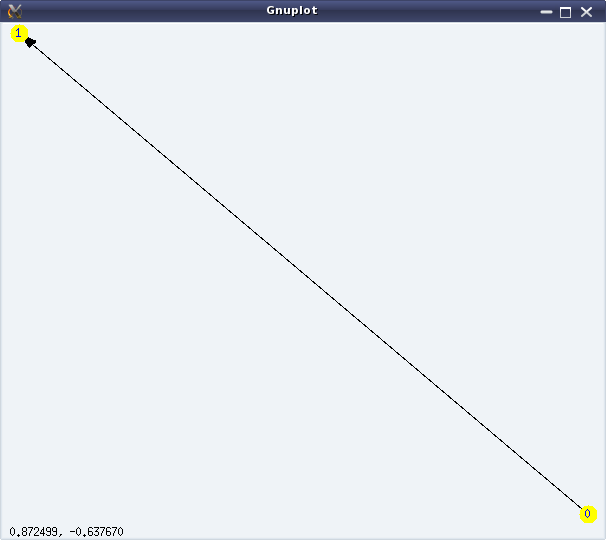
Figure 25: Simple directed graph
Graph creation & visualization
Now, how did we get those figures? Using the graphs package of Maxima, which is loaded by invoking load(graphs) at the Maxima prompt. In the package, vertices are represented by whole numbers 0, 1, … and an edge is represented as a list of its two vertices. Using these notations, we can create graphs using the create_graph(<vertex_list>, <edge_list>[, directed]) function. And, then draw_graph(<graph>[, <option1>, <option2>, …]) would draw the graph pictorially. Code snippet below shows the same in action:
$ maxima -q
(%i1) load(graphs)$
...
0 errors, 0 warnings
(%i2) g: create_graph([0, 1], [[0, 1]])$
(%i3) dg: create_graph([0, 1], [[0, 1]], directed=true)$
(%i4) draw_graph(g, show_id=true, vertex_size=5, vertex_color=yellow)$
(%i5) draw_graph(dg, show_id=true, vertex_size=5, vertex_color=yellow)$
The “show_id=true” option draws the vertex numbers, and vertex_size and vertex_color draws the vertices with the corresponding size and colour.
Note that a graph without any duplicate edges and without any loops is called a simple graph. And, an edge from a vertex U to V is not duplicate of an edge from vertex V to U in a directed graph but is duplicate in an undirected graph. Maxima’s package supports only simple graphs, i.e. graphs without duplicate edges and loops.
A simple graph can also be equivalently represented by adjacency of vertices, meaning by lists of adjacent vertices for every vertex. print_graph(<graph>) exactly displays those lists. The following code demonstration, in continuation from the previous code, demonstrates that:
(%i6) print_graph(g)$

Graph on 2 vertices with 1 edges.
Adjacencies:
  1 :  0
  0 :  1
(%i7) print_graph(dg)$

Digraph on 2 vertices with 1 arcs.
Adjacencies:
  1 :
  0 :  1
(%i8) quit();
create_graph(<num_of_vertices>, <edge_list>[, directed]) is another way of creating a graph using create_graph(). Here, the vertices are created as 0, 1, …, <num_of_vertices> – 1. So, both the above graphs could equivalently be created as follows:
$ maxima -q
(%i1) load(graphs)$
...
0 errors, 0 warnings
(%i2) g: create_graph(2, [[0, 1]]);
(%o2)                     GRAPH(2 vertices, 1 edges)
(%i3) dg: create_graph(2, [[0, 1]], directed=true);
(%o3)                     DIGRAPH(2 vertices, 1 arcs)
(%i4) quit();
make_graph(<vertices>, <predicate>[, directed]) is another interesting way of creating a graph, based on vertex connectivity conditions specified by the <predicate> function. <vertices> could be an integer or a set/list of vertices. If it is a positive integer, then the vertices would be 1, 2, …, <vertices>. In any case, <predicate> should be a function taking two arguments of the vertex type and returning true or false. make_graph() creates a graph with the vertices specified as above, and with the edges between the vertices for which the <predicate> function returns true.
A trivial case would be, if the <predicate> always returns true, then it would create a complete graph, i.e. a simple graph where all vertices are connected to each other. Here are a couple of demonstrations of make_graph():
$ maxima -q
(%i1) load(graphs)$
...
0 errors, 0 warnings
(%i2) f(i, j) := true$
(%i3) g: make_graph(6, f);
(%o3)                   GRAPH(6 vertices, 15 edges)
(%i4) draw_graph(g, show_id=true, vertex_color=yellow)$
(%i5) f(i, j) := is(mod(i, j)=0)$
(%i6) g: make_graph(10, f, directed = true);
(%o6)                  DIGRAPH(10 vertices, 17 arcs)
(%i7) draw_graph(g, show_id=true, vertex_color=yellow, vertex_size=4)$
(%i8) quit();
Figures 26 shows the output graphs from the above code.
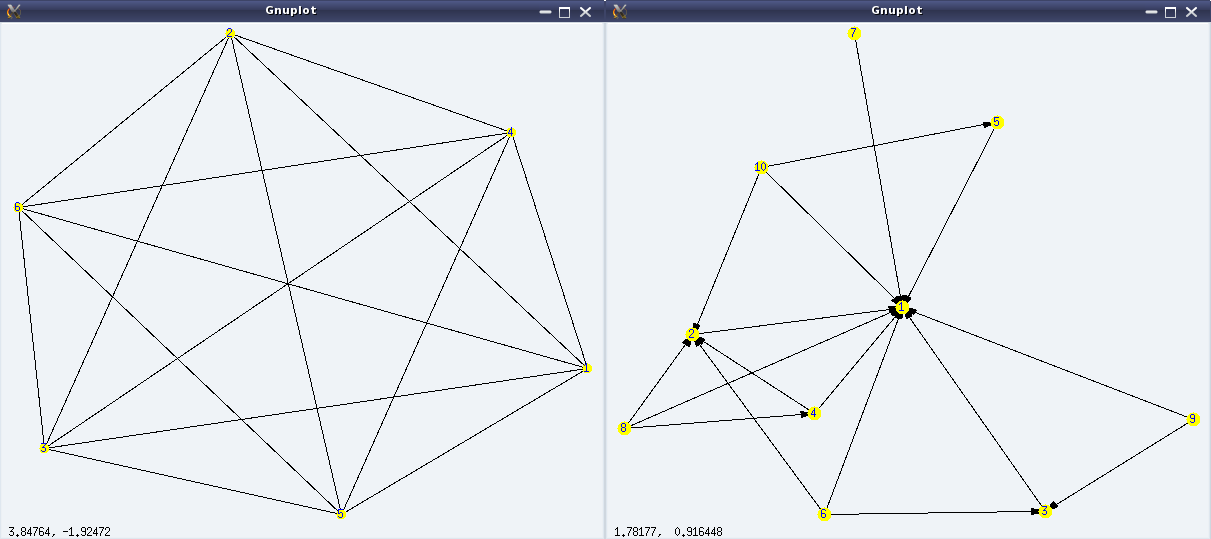
Figure 26: More simple graphs
Graph varieties
One aware of graphs, would have known or at least heard of a variety of them. Here’s a list of some of them, available in Maxima’s graphs package (through functions):
- Empty graph (empty_graph(n)) – Graph with a given n vertices but no edges
- Complete graph (complete_graph(n)) – Simple graph with all possible edges for a given n vertices
- Complete bipartite graph (complete_bipartite_graph(m, n)) – Simple graph with two set of vertices, having all possible edges between the vertices from the two sets, but with no edge between the vertices of the same set.
- Cube graph (cube_graph(n)) – Graph representing an n-dimensional cube
- Dodecahedron graph (dodecahedron_graph()) – Graph forming a 3-D polyhedron with 12 pentagonal faces
- Cuboctahedron graph (cuboctahedron_graph()) – Graph forming a 3-D polyhedron with 8 triangular faces and 12 square faces
- Icosahedron graph (icosahedron_graph()) – Graph forming a 3-D polyhedron with 20 triangular faces
- Icosidodecahedron graph (icosidodecahedron_graph()) – Graph forming a 3-D uniform star polyhedron with 12 star faces and 20 triangular faces
And here follows a demonstration of the above, along with the visuals (left to right, top to bottom) in Figure 27:
$ maxima -q
(%i1) load(graphs)$
...
0 errors, 0 warnings
(%i2) g: empty_graph(5);
(%o2)                     GRAPH(5 vertices, 0 edges)
(%i3) draw_graph(g, show_id=true, vertex_color=yellow)$
(%i4) g: complete_graph(5);
(%o4)                     GRAPH(5 vertices, 10 edges)
(%i5) draw_graph(g, show_id=true, vertex_color=yellow)$
(%i6) g: complete_bipartite_graph(5, 3);
(%o6)                     GRAPH(8 vertices, 15 edges)
(%i7) draw_graph(g, show_id=true, vertex_color=yellow)$
(%i8) g: cube_graph(3);
(%o8)                    GRAPH(8 vertices, 12 edges)
(%i9) draw_graph(g, show_id=true, vertex_color=yellow)$
(%i10) g: cube_graph(4);
(%o10)                   GRAPH(16 vertices, 32 edges)
(%i11) draw_graph(g, show_id=true, vertex_color=yellow)$
(%i12) g: dodecahedron_graph();
(%o12)                   GRAPH(20 vertices, 30 edges)
(%i13) draw_graph(g, show_id=true, vertex_color=yellow)$
(%i14) g: cuboctahedron_graph();
(%o14)                   GRAPH(12 vertices, 24 edges)
(%i15) draw_graph(g, show_id=true, vertex_color=yellow)$
(%i16) g: icosahedron_graph();
(%o16)                   GRAPH(12 vertices, 30 edges)
(%i17) draw_graph(g, show_id=true, vertex_color=yellow)$
(%i18) g: icosidodecahedron_graph();
(%o18)                   GRAPH(30 vertices, 60 edges)
(%i19) draw_graph(g, show_id=true, vertex_color=yellow)$
(%i20) quit();
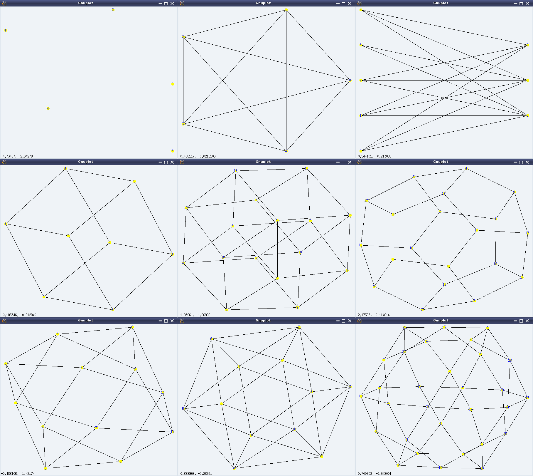
Figure 27: Graph varieties
Graph beauties
Graphs are really beautiful to visualize. Some of the many beautiful graphs, available in Maxima’s graphs package (through functions), are listed below:
- Circulant graph (circulant_graph(n, [x, y, …])) – Graph with vertices 0, …, n-1, where every vertex is adjacent to its xth, yth, … vertices. Visually, it has a cyclic group of symmetries./li>
- Flower graph (flower_snark(n)) – Graph like a flower with n petals and 4*n vertices
- Wheel graph (wheel_graph(n)) – Graph like a wheel with n vertices
- Clebsch graph (clebsch_graph()) – An another symmetrical graph beauty, named by J J Seidel
- Frucht graph (frucht_graph()) – A graph with 12 vertices, 18 edges, and no nontrivial symmetries, such that every vertex have 3 neighbours. It is named after Robert Frucht
- Grötzsch graph (grotzch_graph()) – A triangle-free graph with 11 vertices and 20 edges, named after Herbert Grötzsch
- Heawood graph (heawood_graph()) – A symmetrical graph with 14 vertices and 21 edges, named after Percy John Heawood
- Petersen graph (petersen_graph()) – A symmetrical graph with 10 vertices and 15 edges, named after Julius Petersen
- Tutte graph (tutte_graph()) – A graph with 46 vertices and 69 edges, such that every vertex have 3 neighbours. It is named after W T Tutte
And here follows a demonstration of some of the above, along with the visuals (left to right, top to bottom) in Figure 28:
$ maxima -q
(%i1) load(graphs)$
...
0 errors, 0 warnings
(%i2) g: circulant_graph(10, [1, 3]);
(%o2)                   GRAPH(10 vertices, 20 edges)
(%i3) draw_graph(g, show_id=true, vertex_color=yellow)$
(%i4) g: circulant_graph(10, [1, 3, 4, 6]);
(%o4)                   GRAPH(10 vertices, 40 edges)
(%i5) draw_graph(g, show_id=true, vertex_color=yellow)$
(%i6) g: flower_snark(3);
(%o6)                   GRAPH(12 vertices, 18 edges)
(%i7) draw_graph(g, show_id=true, vertex_color=yellow)$
(%i8) g: flower_snark(5);
(%o8)                   GRAPH(20 vertices, 30 edges)
(%i9) draw_graph(g, show_id=true, vertex_color=yellow)$
(%i10) g: flower_snark(8);
(%o10)                   GRAPH(32 vertices, 48 edges)
(%i11) draw_graph(g, show_id=true, vertex_color=yellow)$
(%i12) g: flower_snark(10);
(%o12)                   GRAPH(40 vertices, 60 edges)
(%i13) draw_graph(g, show_id=true, vertex_color=yellow)$
(%i14) g: wheel_graph(3);
(%o14)                    GRAPH(4 vertices, 6 edges)
(%i15) draw_graph(g, show_id=true, vertex_color=yellow)$
(%i16) g: wheel_graph(4);
(%o16)                    GRAPH(5 vertices, 8 edges)
(%i17) draw_graph(g, show_id=true, vertex_color=yellow)$
(%i18) g: wheel_graph(5);
(%o18)                    GRAPH(6 vertices, 10 edges)
(%i19) draw_graph(g, show_id=true, vertex_color=yellow)$
(%i20) g: wheel_graph(10);
(%o20)                   GRAPH(11 vertices, 20 edges)
(%i21) draw_graph(g, show_id=true, vertex_color=yellow)$
(%i22) g: wheel_graph(100);
(%o22)                  GRAPH(101 vertices, 200 edges)
(%i23) draw_graph(g, show_id=true, vertex_color=yellow)$
(%i24) g: clebsch_graph();
(%o24)                   GRAPH(16 vertices, 40 edges)
(%i25) draw_graph(g, show_id=true, vertex_color=yellow)$
(%i26) g: grotzch_graph();
(%o26)                   GRAPH(11 vertices, 20 edges)
(%i27) draw_graph(g, show_id=true, vertex_color=yellow)$
(%i28) g: petersen_graph();
(%o28)                   GRAPH(10 vertices, 15 edges)
(%i29) draw_graph(g, show_id=true, vertex_color=yellow)$
(%i30) g: tutte_graph();
(%o30)                   GRAPH(46 vertices, 69 edges)
(%i31) draw_graph(g, show_id=true, vertex_color=yellow)$
(%i32) quit();
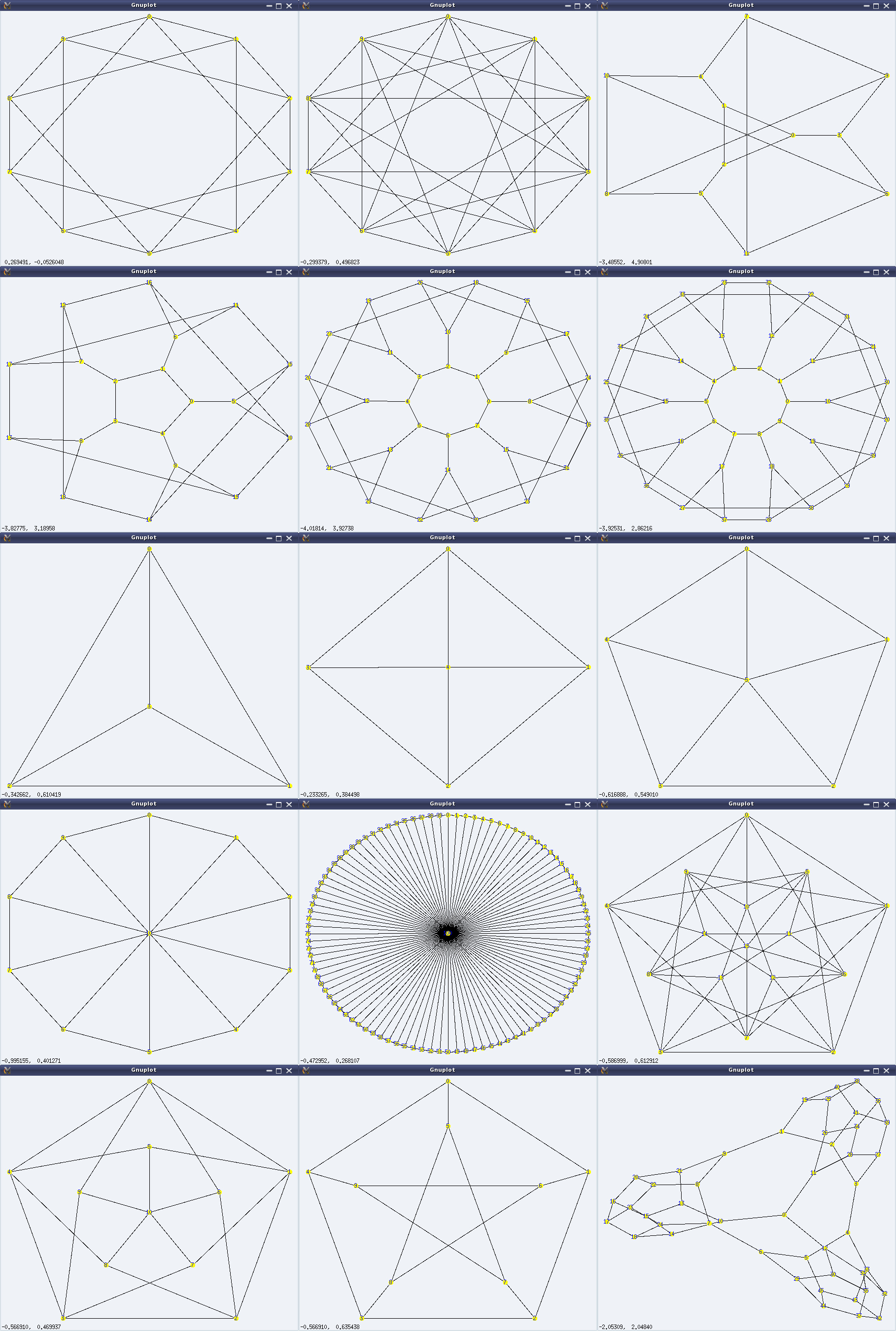
Figure 28: Graph beauties
What next?
With all these visualizations, you may be wondering, what to do with these apart from just staring at them. Visualizations were just to motivate you, visually. In fact, every graph has a particular set of properties, which distinguishes it from the other. And, there is a lot of beautiful mathematics involved with these properties. If you are motivated enough, watch out for playing around with these graphs and their properties.