Monthly Archives: December 2013

USB Drivers in Linux

This eleventh article, which is part of the series on Linux device drivers, gets you started with writing your first USB driver in Linux.

<< Tenth Article

Pugs’ pen drive was the device, Shweta was playing with, when both of them sat down to explore the world of USB drivers in Linux. The fastest way to get hang of one, the usual Pugs’ way, was to pick up a USB device and write a driver for it to experiment with. So, they chose pen drive aka USB stick, available at hand. It was JetFlash from Transcend with vendor ID 0x058f and product ID 0x6387.

USB device detection in Linux

Whether a driver of a USB device is there or not on a Linux system, a valid USB device would always get detected at the hardware and kernel spaces of a USB-enabled Linux system. A valid USB device is a device designed and detected as per USB protocol specifications. Hardware space detection is done by the USB host controller – typically a native bus device, e.g. a PCI device on x86 systems. The corresponding host controller driver would pick and translate the low-level physical layer information into higher level USB protocol specific information. The USB protocol formatted information about the USB device is then populated into the generic USB core layer (usbcore driver) in the kernel space, thus enabling the detection of a USB device in the kernel space, even without having its specific driver.

After this, it is up to the various drivers, interfaces, and applications (which are dependent on the various Linux distributions), to have the user space view of the detected devices. Figure 17 shows a top to bottom view of USB subsystem in Linux. A basic listing of all detected USB devices can be obtained using the lsusb command, as root. Figure 18 shows the same, without and with the pen drive being inserted into the system. A -v option to lsusb provides detailed information. In many Linux distributions like Mandriva, Fedora, … usbfs driver is loaded as part of the default configuration. This enables the detected USB device details to be viewed in a more techno-friendly way through the /proc window using cat /proc/bus/usb/devices. Figure 19 shows a typical snippet of the same, clipped around the pen drive specific section. The complete listing basically contains such sections, each for one of the valid USB devices detected on the Linux system.

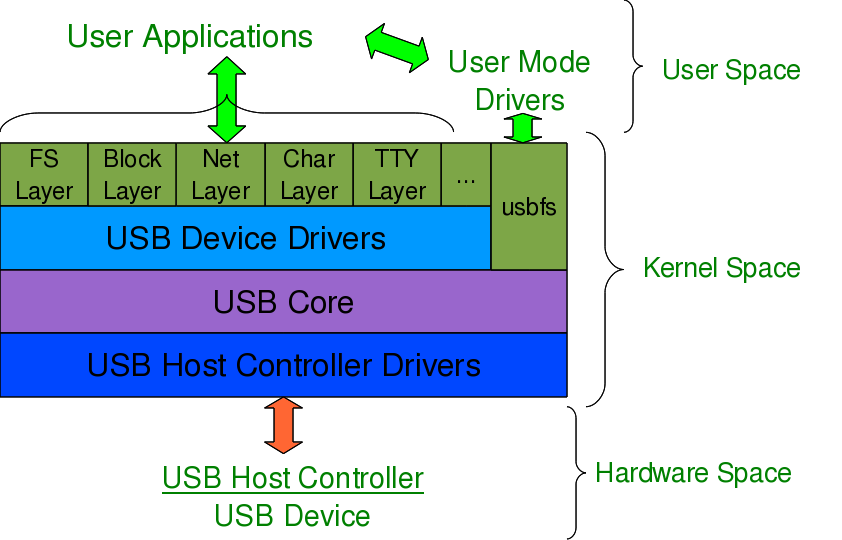
Figure 17: USB subsystem in Linux

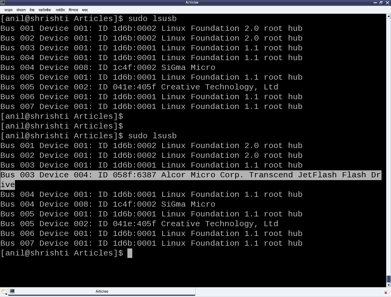
Figure 18: Output of lsusb

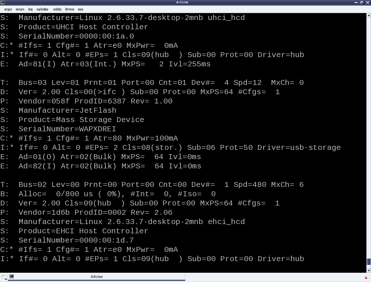
Figure 19: USB’s proc window snippet

Decoding a USB device section

To further decode these sections, a valid USB device needs to be understood first. All valid USB devices contain one or more configurations. A configuration of a USB device is like a profile, where the default one is the commonly used one. As such, Linux supports only one configuration per device – the default one. For every configuration, the device may have one or more interfaces. An interface corresponds to the functionality provided by the device. There would be as many interfaces as the number of independent functionalities provided by the device. So, say an MFD (multi-function device) USB printer can do printing, scanning, and faxing, then it most likely would have at least three interfaces – one for each of the functionalities. So, unlike other device drivers, a USB device driver is typically associated/written per interface, rather than the device as a whole – meaning one USB device may have multiple device drivers. Though definitely one interface can have a maximum of one driver only.

Moreover, it is okay and common to have a single USB device driver for all the interfaces of a USB device. The “Driver=…” entry in the proc window output (Figure 19) shows the interface is to driver mapping – a “(none)” indicating no associated driver. For every interface, there would be one or more end points. An endpoint is like a pipe for transferring information either into or from the interface of the device, depending on the functionality. Depending on the type of information, the endpoints have four types:

Control
Interrupt
Bulk
Isochronous

As per USB protocol specification, all valid USB devices have an implicit special control endpoint zero, the only bi-directional endpoint. Figure 20 shows the complete pictorial representation of a valid USB device, based on the above explanation.

Coming back to the USB device sections (Figure 19), the first letter on each line represents the various parts of the USB device specification just explained. For example, D for device, C for configuration, I for interface, E for endpoint, etc. Details about them and various others are available under the kernel source Documentation/usb/proc_usb_info.txt

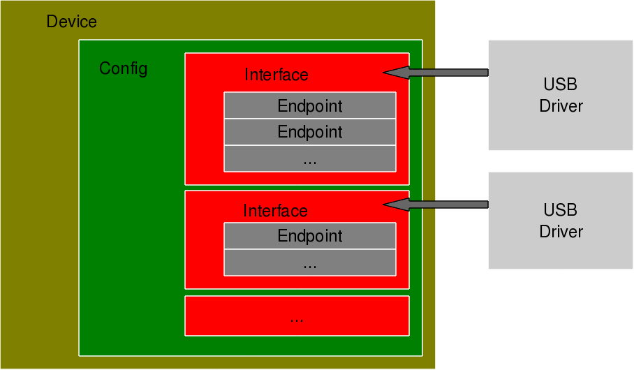
Figure 20: USB device overview

The USB pen drive driver registration

“Seems like there are so many things to know about the USB protocol to be able to write the first USB driver itself – device configuration, interfaces, transfer pipes, their four types, and so many other symbols like T, B, S, … under a USB device specification”, sighed Shweta. “Yes, but don’t you worry – all these can be talked in detail, later. Let’s do the first thing first – get our pen drive’s interface associated with our USB device driver (pen_register.ko)”, consoled Pugs. Like any other Linux device driver, here also we need the constructor and the destructor – basically the same driver template that has been used for all the drivers. Though the content would vary as this is a hardware protocol layer driver, i.e. a horizontal driver unlike a character driver, which was one of the vertical drivers, discussed so far. And the difference would be that instead of registering with & unregistering from VFS, here we would do that with the corresponding protocol layer – the USB core in this case; instead of providing a user space interface like a device file, it would get connected with the actual device in the hardware space. The USB core APIs for the same are as follows (prototyped in <linux/usb.h>):

int usb_register(struct usb_driver *driver);
void usb_deregister(struct usb_driver *);

As part of the usb_driver structure, the fields to be provided are the driver’s name, ID table for auto-detecting the particular device and the 2 callback functions to be invoked by USB core during hot-plugging and hot-removal of the device, respectively. Putting it all together, pen_register.c would look like:

#include <linux/module.h>
#include <linux/kernel.h>
#include <linux/usb.h>

static int pen_probe(struct usb_interface *interface, const struct usb_device_id *id)
{
	printk(KERN_INFO "Pen drive (%04X:%04X) plugged\n", id->idVendor,
								id->idProduct);
	return 0;
}

static void pen_disconnect(struct usb_interface *interface)
{
	printk(KERN_INFO "Pen drive removed\n");
}

static struct usb_device_id pen_table[] =
{
	{ USB_DEVICE(0x058F, 0x6387) },
	{} /* Terminating entry */
};
MODULE_DEVICE_TABLE (usb, pen_table);

static struct usb_driver pen_driver =
{
	.name = "pen_driver",
	.id_table = pen_table,
	.probe = pen_probe,
	.disconnect = pen_disconnect,
};

static int __init pen_init(void)
{
	return usb_register(&pen_driver);
}

static void __exit pen_exit(void)
{
	usb_deregister(&pen_driver);
}

module_init(pen_init);
module_exit(pen_exit);

MODULE_LICENSE("GPL");
MODULE_AUTHOR("Anil Kumar Pugalia <email@sarika-pugs.com>");
MODULE_DESCRIPTION("USB Pen Registration Driver");

Then, the usual steps for any Linux device driver may be repeated:

Build the driver (.ko file) by running make
Load the driver using insmod
List the loaded modules using lsmod
Unload the driver using rmmod

But surprisingly the results wouldn’t be as expected. Check for dmesg and the proc window to see the various logs and details. Not because USB driver is different from a character driver. But there’s a catch. Figure 19 shows that the pen drive has one interface (numbered 0), which is already associated with the usual usb-storage driver. Now, in order to get our driver associated with that interface, we need to unload the usb-storage driver (i.e. rmmod usb-storage) after plugging in the pen drive, and then load our driver. Once this sequence is followed, the results would be as expected. Figure 21 shows a glimpse of the possible logs and proc window snippet. Repeat hot-plugging in and hot-plugging out the pen drive to observe the probe and disconnect calls in action – but don’t forget unloading the usb-storage driver, every time you plug in the pen driver.

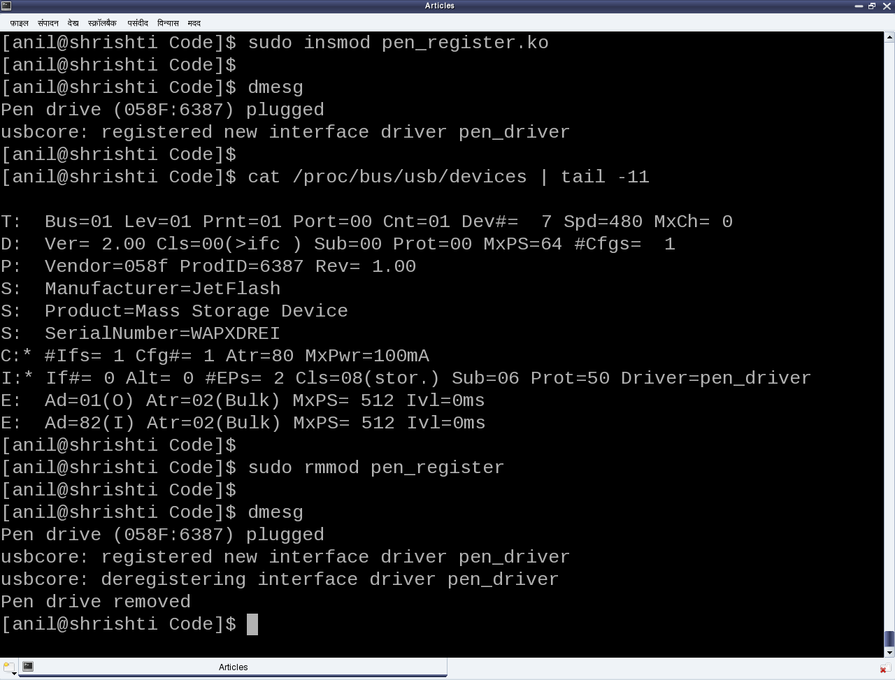
Figure 21: Pen driver in action

Summing up

“Finally!!! Something into action.”, relieved Shweta. “But seems like there are so many things around (like the device ID table, probe, disconnect, …), yet to be assimilated and understood to get a complete USB device driver, in place”, she continued. “Yes, you are right. Let’s take them one by one, with breaks”, replied Pugs taking a stretching break.

Twelfth Article >>

Notes

Make sure that you replace the vendor id & device id in the above code examples by the ones of your pen drive.
One may wonder, as how does the usb-storage get autoloaded. The answer lies in the module autoload rules written down in the file /lib/modules/<kernel_version>/modules.usbmap. If you are an expert, you may comment out the corresponding line, for it to not get autoloaded. And uncomment it back, once you are done with your experiments.
In latest distros, you may not find the detailed description of the USB devices using cat /proc/bus/usb/devices, as the /proc/bus/usb/ itself has been deprecated. You can find the same detailed info using cat /sys/kernel/debug/usb/devices – though you may need root permissions for the same. Also, if you do not see any file under /sys/kernel/debug (even as root), then you may have to first mount the debug filesystem, as follows: mount -t debugfs none /sys/kernel/debug

Polynomial Curve Fitting & Interpolation

2 Replies

This eleventh article of the mathematical journey through open source, explains curve fitting & interpolation with polynomials in octave.

<< Tenth Article

In various fields of physics, chemistry, statistics, economics, … we very often come across something called curve fitting, and interpolation.

Given a set of data points from our observations, we would like to see what mathematical equation does they follow. So, we try to fit the best curve through those data points, called the curve fitting technique. Once we have the equation, the main advantage is that then we can find the values at the points, we haven’t observed by just substituting that value in the equation. One may think of this as interpolation. But this is not exactly interpolation. As in interpolation, we are restricted to finding unobserved values only between two observed points, using a pre-defined curve fit between those two points. With that we may not be able to get values outside our observation range. But the main reason for using that is when we are not interested or it is not meaningful or we are unable to fit a known form of curve in the overall data set, but still we want to get some approximations of values, in between the observed data points. Enough of gyaan, now let’s look into each one of those.

Curve Fitting

Let’s say for any system, we have the following data points:
For the inputs of 1, 3, 6, 10, 20, we get the outputs as 2.5, 7.5, 15.5, 24, 45, respectively. Then, we would like to know as how is input is related to the output. So, to get a feel of the relation, we first plot this points on a x-y plane, say inputs as x and outputs as y. Figure 6 shows the same. And the octave code for that is as follows:

$ octave -qf
octave:1> x = [1 3 6 10 20];
octave:2> y = [2.5 7.5 15.5 24 45];
octave:3> plot(x, y, "*");
octave:4> xlabel("Inputs");
octave:5> ylabel("Outputs");
octave:6>

Figure 6: Plot of the data points

By observing the plot, the simplest fitting relation looks to be a straight line. So, let’s try fitting a linear polynomial, i.e. a first order polynomial, i.e. a straight line. Here’s the code in execution for it:

octave:1> x = [1 3 6 10 20];
octave:2> y = [2.5 7.5 15.5 24 45];
octave:3> p = polyfit(x, y, 1)
p =

   2.2212   1.1301

octave:4> polyout(p, "x");

2.2212*x^1 + 1.1301

octave:5> plot(x, y, "*", x, polyval(p, x), "-");
octave:6> xlabel("Inputs");
octave:7> ylabel("Outputs");
octave:8> legend("Data points", "Linear Fit");
octave:9>

polyfit() takes 3 arguments, the x values, the y values, and the order of the polynomial to fit – 1 for linear. It then returns the coefficients of the fitted polynomial p. polyout() displays the polynomial in more readable format. So, the fitted equation is y = 2.2212 * x + 1.1301. polyval() takes the polynomial p and the input values x, and calculates the output values y, as per the polynomial equation. And then we plot them, along with the earlier data points, on the same plot. Figure 7 shows the same, 2.2212 being the slope / gradient of the straight line, and 1.1301 being the intercept. Now, we notice that the straight line does not fit exactly, and there is some deviation from the observed points. polyfit() fits the polynomial with the minimum deviation for the order we request, but still there is a deviation, as that is the minimum possible. If you want to get the standard deviation for the particular fit, you just need to do the following:

octave:9> std_dev = sqrt(mean((y - polyval(p, x)).^2))
std_dev =  0.72637
octave:10>

Figure 7: Linear fit of data points

And we see that it is a small value compared to our output values. But say we are not fully satisfied with this, we may like to try higher order polynomials, say of order 2, a quadratic, and observe the results from it. Here’s how one would do this:

octave:1> x = [1 3 6 10 20];
octave:2> y = [2.5 7.5 15.5 24 45];
octave:3> p = polyfit(x, y, 2)
p =

  -0.018639   2.623382  -0.051663

octave:4> polyout(p, "x");

-0.018639*x^2 + 2.6234*x^1 - 0.051663

octave:5> plot(x, y, "*", x, polyval(p, x), "-");
octave:6> xlabel("Inputs");
octave:7> ylabel("Outputs");
octave:8> legend("Data points", "Quadratic Fit");
octave:9> std_dev = sqrt(mean((y - polyval(p, x)).^2))
std_dev =  0.26873
octave:10>

Figure 8 shows the data points and fitted quadratic curve. All the values above can be interpreted in the similar way as earlier. And we note that the standard deviation has come down further. In fact, as we increase the polynomial order further and further, we will definitely note that the standard deviation keeps on decreasing, till the order is same as number of data points – 1, after which it remains 0. But, we may not like to do this, as our observed data points are typically not perfect, and we are typically not interested in getting the standard deviation zero but for a fit more appropriate to reflect the relation between the system’s input and output.

Figure 8: Quadratic fit of data points

Interpolation

Now, say we have the following wierd data points, listed as (x, y) pairs: (1, 1), (2, 2), (3, 3), (4, 2), (5, 1), (6, 3.75), (7, 7), (8, 3), (9, 0), (11, 8). Figure 9 shows, how wierd they look like.

Figure 9: Wierd data points

Trying to fit a polynomial, would be quite meaningless. But still they seem to have some correlation in between smaller ranges of input, say between 1 and 3, 3 and 5, 5 and 7, and so on. So, this is best suited for us to do interpolation for finding the values in between, say at 1.5, 3.8, 10, … Now interpolation is all about curve fitting between two neighbouring data points and then calculating the value at any intermediate point. So, the typical varieties of techniques used for this “piece-wise curve fitting” are:

nearest: Return the nearest data point (actually no curve fitting)
linear: Linear/Straight line fitting between the two neighbouring data points
pchip: Piece-wise cubic (order 3) hermite polynomial fitting
cubic: Cubic (order 3) polynomial fitted between four nearest neighbouring data points
spline: Cubic (order 3) spline fitting with smooth first and second derivatives throughout the curve

All these may look little jargonish – so don’t worry about that. Let’s just try out some examples to drive the point home. Here’s the code to show the nearest & linear interpolation for the above data:

octave:1> x = [1 2 3 4 5 6 7 8 9 11];
octave:2> y = [1 2 3 2 1 3.75 7 3 0 8];
octave:3> xi = 1:0.1:11;
octave:4> y_n = interp1(x, y, xi, "nearest");
octave:5> y_l = interp1(x, y, xi, "linear");
octave:6> plot(x, y, "*", xi, y_n, "-", xi, y_l, "-");
octave:7> xlabel("Inputs");
octave:8> ylabel("Outputs");
octave:9> legend("Data points", "Nearest", "Linear");
octave:10>

Figure 10 shows the same.

Figure 10: Nearest and linear interpolations of the data points

Now, if we want to get the interpolated values say at the points 1.5, 3.8, 10, instead of giving all the intermediate points xi in the above code, we may just give these 3 – that’s all. Here goes the code in execution for the that:

octave:1> x = [1 2 3 4 5 6 7 8 9 11];
octave:2> y = [1 2 3 2 1 3.75 7 3 0 8];
octave:3> our_x = [1.5 3.8 10];
octave:4> our_y_n = interp1(x, y, our_x, "nearest")
our_y_n =

   2   2   8

octave:5> our_y_l = interp1(x, y, our_x, "linear")
our_y_l =

   1.5000   2.2000   4.0000

octave:6>

Now, before closing on interpolation, just to give a feel of all of the interpolation techniques, here goes an example with the points on a sine curve:

octave:1> x = 0:2*pi;
octave:2> y = sin(x);
octave:3> xi = 0:0.1:2*pi;
octave:4> y_n = interp1(x, y, xi, "nearest");
octave:5> y_l = interp1(x, y, xi, "linear");
octave:6> y_p = interp1(x, y, xi, "pchip");
octave:7> y_c = interp1(x, y, xi, "cubic");
octave:8> y_s = interp1(x, y, xi, "spline");
octave:9> plot(x, y, "*", xi, y_n, "-", xi, y_l, "-", xi, y_p, "-", xi, y_c, "-",
                                                                      xi, y_s, "-");
octave:10> xlabel("x ->");
octave:11> ylabel("y ->");
octave:12> legend("Data points", "Nearest", "Linear", "Pchip", "Cubic", "Spline");
octave:13> print("-dpng", "all_types_of_interpolations.png");
octave:14>

Figure 11 shows the visualization of the same for your eyes.

Figure 11: All types of interpolations for sinusoidal points

What’s next?

With today’s curve fitting & interpolation walk through, we have used some basic 2-D plotting techniques. But there are many more features and techniques to plotting, like marking our plots, visualizing 3-D stuff, etc. Next, we’ll look into that.