This thirteenth article of the mathematical journey through open source, gives a glimpse of statistical capabilities of octave.
Statistics – the name itself brings to the mind the thought of data, and the associated probabilities, averages, deviations, random numbers. Rather than getting perplexed by all these, octave shows out how to use them in a very conducive way.
Data moments
Already got scared by the name itself. Don’t worry. Moments basically mean the various kinds of averages, median, modes, etc. To understand them, let’s take some random data set, which may be generated using any of the various distributions. Let’s take the most “natural” normal distribution – yes the bell-shaped one. Figure 19 shows one centered around 0 (the mean) with a spread of 3 (the standard deviation), generated using normpdf(), as cited below. Note that octave has a whole set of all such functions.
$ octave -qf
octave:1> X = -10:0.1:10;
octave:2> Y = normpdf(X, 0, 3); # Normal Density Function
octave:3> plot(X, Y, "b*");
octave:4> xlabel("X ->");
octave:5> ylabel("Y = e^{-{x^2}/3} ->");
octave:6> title("Normal Distribution");
octave:7> grid("on");
octave:8>
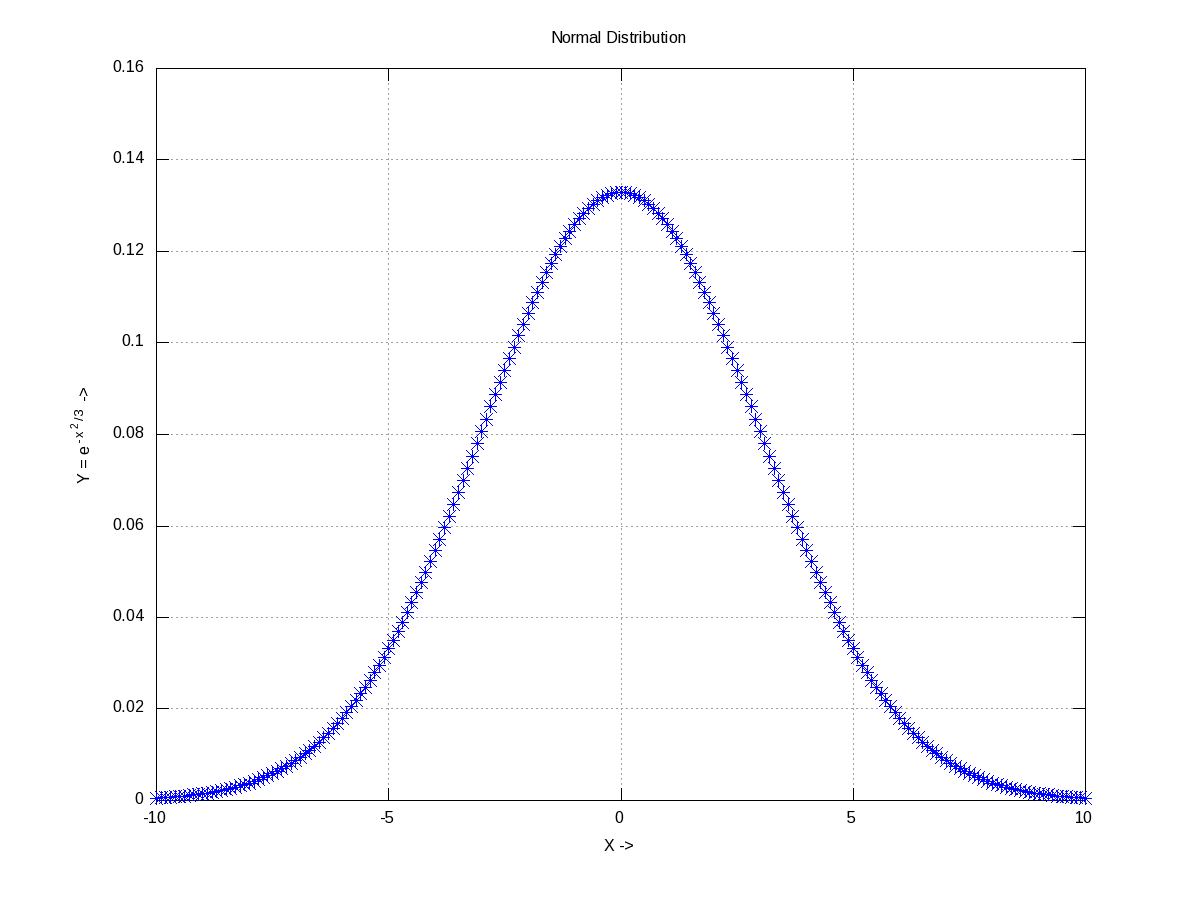
Figure 19: Normal distribution with mean = 0, std = 3
If we take all the infinite points on this curve, would get a mean of 0 and a standard deviation of 3. But that’s not practical. So, let’s pick, say 10 random points from it. normrnd(m, s, 10, 1) provides the same in a 10×1 vector, following the normal distribution of mean m & standard deviation s. And then, mean() & std() give the mean and standard deviation, respectively. mean() could be of three types: Ordinary (arithmetic) mean (“a”), Geometric mean (“g”), Harmonic mean (“h”).
$ octave -qf
octave:1> Y = normrnd(0, 3, 10, 1) # m=0; s=3; 10x1 vector
Y =

  -2.33218
  -3.16866
   3.41991
  -2.27566
  -1.45403
   7.79691
   2.12849
   2.32727
  -5.37920
  -0.63447
octave:2> mean(Y)
ans =  0.042839
octave:3> mean(Y, "h")
ans =  -4.3226
octave:4> std(Y)
ans =  3.8662
octave:5> median(Y)
ans = -1.0442
octave:6> cov(Y, Y)
ans =  14.947
octave:7> cor(Y, Y)
ans =  1
octave:8>
Among many other moments, the four common ones are: 1) median() gets the middle most element in the sorted arrangement of data; 2) mode() gets the most frequently occurring data point; 3) cov() gives the variance between two set of data points, i.e. the covariance; 4) cor() gives the relation between two set of data points, i.e. the correlation ranging from -1 to 1. Correlation of 1 indicating they are completely related, 0 indicating totally unrelated, and a -1 indicating related completely but in an opposite sense.
Visualizing the probabilities
Random numbers are a beautiful example of probabilities. They occur as per their probabilities decided by the probability density function (PDF) they follow. Let’s visualize that using a live example. So again, as in the above example, let’s take some random numbers following the normal distribution. But, this time we’ll take a lot more points, say 1,00,000 points, so that we can actually see them following the bell-shape. But still, we are not having infinite points to give the continuous bell. So, what we have to do is collect the random points around some pre-designated buckets of fixed ranges. That is what we call a histogram. histc() does exactly that, returning the number of points in each of the buckets, which we can then plot to see our bell. Another function hist(), does all those in a more beautiful way. Figure 20 shows the two plots, for which the code follows:
$ octave -qf
octave:1> Y=normrnd(0, 3, 100000, 1); # 1 lakh random points
octave:2> B=-10:1:10; # Bucket edges -10, -9, ..., 10, i.e. 21 buckets
octave:3> N=histc(Y, B);
octave:4> subplot(1, 2, 1);
octave:5> plot(B, N, "r*", B, N, "b-");
octave:6> subplot(1, 2, 2);
octave:7> hist(Y, B); # More beautiful boxy plot
octave:8>
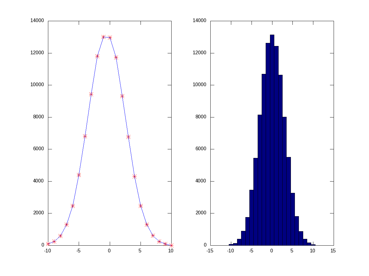
Figure 20: Histograms of normal distributed random points
Similarly, if we use other PDFs, we would see similar histograms for them as well. Figure 21 shows nine such others, namely Beta (with alpha = beta = 0.5), Cauchy, Chi-Square, Exponential, Gamma, Laplace, Log Normal, Poisson, Uniform, using their respective functions, as shown in the code below:
octave:1> B=-20:0.5:20;
octave:2> subplot(3, 3, 1);
octave:3> hist(40*(betarnd(0.5, 0.5, 100000, 1) - 0.5), B);
octave:4> title("Beta");
octave:5> subplot(3, 3, 2);
octave:6> hist(cauchy_rnd(0, 1, 100000, 1), B);
octave:7> title("Cauchy");
octave:8> subplot(3, 3, 3);
octave:9> hist(chi2rnd(5, 100000, 1), B);
octave:10> title("Chi Square");
octave:11> subplot(3, 3, 4);
octave:12> hist(exprnd(5, 100000, 1), B);
octave:13> title("Exponential");
octave:14> subplot(3, 3, 5);
octave:15> hist(gamrnd(5, 1, 100000, 1), B);
octave:16> title("Gamma");
octave:17> subplot(3, 3, 6);
octave:18> hist(laplace_rnd(100000, 1), B);
octave:19> title("Laplace");
octave:20> subplot(3, 3, 7);
octave:21> hist(lognrnd(0, 1, 100000, 1), B);
octave:22> title("Log Normal");
octave:23> subplot(3, 3, 8);
octave:24> hist(poissrnd(5, 100000, 1), B);
octave:25> title("Poisson");
octave:26> subplot(3, 3, 9);
octave:27> hist(unifrnd(-10, 10, 100000, 1), B);
octave:28> title("Uniform");
octave:29>
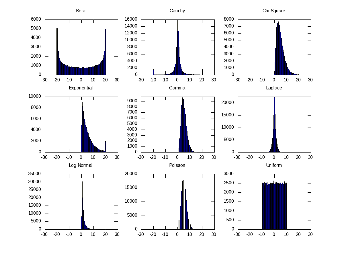
Figure 21: Histograms of probability density functions
Miscellaneous helpers
Apart from the standard ones, discussed so far, there are quite a few miscellaneous useful functions provided by octave. Here are a few:
- perms() – Generates the n! permutations of the data points
- values() – Sorts the data into non-repeating ascending order
- range() – Returns the difference between the maximum and the minimum data points
Here follows a demonstration:
$ octave -qf
octave:1> perms([0 1 2])
ans =

   0   1   2
   1   0   2
   0   2   1
   1   2   0
   2   0   1
   2   1   0

octave:2> values([1 4 -9 -7 0 -6 12 -90])
ans =

  -90
   -9
   -7
   -6
    0
    1
    4
   12

octave:3> range([1 4 -9 -7 0 -6 12 -90])
ans =  102
octave:4>
What’s next?
Till date, in all our mathematical explorations, we have been always dealing with numbers. Ya! So big deal – anyways mathematics is about numbers, only. Not really. Many a times, we come across scenarios, where we would like to solve something symbolically or analytically, and then use numbers only at the end. Such things would not be possible with any of the OSS tools, we have discussed till now. But, yes there are such tools. One such is Maxima. And that’s where we are headed to next.