Mathematics made easy with minimal Octave

This fifth article of the mathematical journey through open source, introduces the minimal, octave can do for you.

You wanted a non-programmers way of doing mathematics and there you go – octave. Sounds like something to do with music, but in reality it is the name the octave author’s chemical engineering professor, who was well know for his ‘back of the envelope’ calculations.

All of bench calculator!!!

All the operations of bench calculator are just a subset of octave. So, no point going round the wheel again. Whatever operations can be done in bc – arithmetic, logical, relational, conditional – all can be done with equal ease in octave. As in bc, it can as well be used as a mathematical programming language. Ha! Then, why did we waste time on learning bc, we could have straight away come to octave. Yes! Yes! Except one thing – the precision-less-ness. We can’t get that in octave. If we need that, we would have to go back to bc. Okay! Fine. So, what with octave – we start with N-dimensions, what else. Hey don’t worry! In simple language, I mean vectors & matrices.

Getting Started

Command: Typing ‘octave‘ on the shell brings up the octave‘s interactive shell. Type ‘quit’ or Control-D to exit. The interactive shell starts with a welcome message. As in bc, we pass option -q for it to not show. Additionally, we’ll use the -f option for it to not pick any local start-up scripts (if any). So, for our examples, the command would look like ‘octave -qf‘ to start octave with an interactive shell.

Prompts & Results: Input prompt is typically denoted by ‘octave:X>‘, where X just a number showing the command count. Valid results are typically shown with ‘<variable> = ‘, or ‘ans = ‘ or ‘=> ‘, and then the command count incremented for the next input. Errors cause error messages to be printed and then octave brings back the input prompt without incrementing the command count. Putting a semicolon (;) at the end of an statement, suppresses it result (return value) to be displayed.

Comments could start with # or %. For block comments, #{ … }# or %{ … }% can be used.

Detailed topic help could be obtained using ‘help <topic>’ or complete documentation using ‘doc’ on the octave shell.

All in a go:

$ octave -qf
octave:1> # This is a comment
octave:1> pi # Built-in constant
ans =  3.1416
octave:2> e # Built-in constant again
ans =  2.7183
octave:3> i # Same as j – the imaginary number
ans =  0 + 1i
octave:4> x = 3^4 + 2*30;
octave:5> x
x =  141
octave:6> y
error: `y' undefined near line 6 column 1
octave:6> doc # Complete doc; Press 'q' to come back
octave:7> help plot # Help on plot
octave:8> A = [1 2 3; 4 5 6; 7 8 9] # 3x3 matrix
A =

   1   2   3
   4   5   6
   7   8   9

octave:9> quit

Matrices with a Heart

Yes, we already saw a matrix in creation. It can also be created through multiple lines. Octave continues waiting for further input by prompting just ‘>’. Checkout below for creating the 3×3 magic square matrix in the same way, followed by various other interesting operations:

$ octave -qf
octave:1> M = [ # 3x3 magic square
> 8 1 6
> 3 5 7
> 4 9 2
> ]
M =

   8   1   6
   3   5   7
   4   9   2

octave:2> B = rand(3, 4); # 3x4 matrix w/ randoms in [0 1]
octave:3> B
B =

   0.068885   0.885998   0.542059   0.797678
   0.652617   0.904360   0.036035   0.737404
   0.043852   0.579838   0.709194   0.053118

octave:4> B' # Transpose of B
ans =

   0.068885   0.652617   0.043852
   0.885998   0.904360   0.579838
   0.542059   0.036035   0.709194
   0.797678   0.737404   0.053118

octave:5> A = inv(M) # Inverse of M
A =

   0.147222  -0.144444   0.063889
  -0.061111   0.022222   0.105556
  -0.019444   0.188889  -0.102778

octave:6> M * A # Should be identity, at least approx.
ans =

   1.00000   0.00000  -0.00000
  -0.00000   1.00000   0.00000
   0.00000   0.00000   1.00000

octave:7> function rv = psine(x) # Our phase shifted sine
>
> rv = sin(x + pi / 6);
>
>  endfunction 
octave:8> x = linspace(0, 2*pi, 400); # 400 pts from 0 to 2*pi
octave:9> plot(x, psine(x)) # Our function's plot
octave:10> polar(x, 10 * (1 - sin(x)), 'm*') # bonus Heart
octave:11> quit

Figure 1 shows the plot window which pops up by the command # 9 – plot.

Figure 2 is the bonus magenta heart of stars (*) from polar coordinates draw command # 10 – polar.

Figure 1: Plot of our 30° phase shifted sine

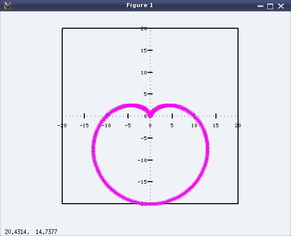
Figure 2: The Heart

What next?

With ready-to-go level of introduction to octave, we are all set to explore it the fun way. What fun? Next one left to your imagination. And as we move on, we would take up one or more fun challenge(s), and try to see, how we solve it using octave.

Sixth Article >>

Anil Kumar Pugalia (123 Posts)

The author is a hobbyist in open source hardware and software, with a passion for mathematics, and philosopher in thoughts. A gold medallist from the Indian Institute of Science, Linux, mathematics and knowledge sharing are few of his passions. He experiments with Linux and embedded systems to share his learnings through his weekend workshops. Learn more about him and his experiments at https://sysplay.in.