This nineteenth article, which is part of the series on Linux device drivers, continues with introducing the concept of a file system, by simulating one in user space.
In the previous article, Shweta readied the partition on the .sfsf file by formating it with the format_sfs application. To complete the understanding of a file system, the next step in its simulation is to browse and play around with the file system created. Here is Shweta’s first-cut browser application to achieve the same. Let’s have a closer look. sfs_ds.h is the same header file, already created by Shweta.
#include <stdio.h>
#include <sys/types.h>
#include <sys/stat.h>
#include <fcntl.h>
#include <unistd.h>
#include <string.h>
#include <time.h>

#include "sfs_ds.h"

sfs_super_block_t sb;

void sfs_list(int sfs_handle)
{
	int i;
	sfs_file_entry_t fe;

	lseek(sfs_handle, sb.entry_table_block_start * sb.block_size, SEEK_SET);
	for (i = 0; i < sb.entry_count; i++)
	{
		read(sfs_handle, &fe, sizeof(sfs_file_entry_t));
		if (!fe.name[0]) continue;
		printf("%-15s  %10d bytes  %c%c%c  %s",
			fe.name, fe.size,
			fe.perms & 04 ? 'r' : '-',
			fe.perms & 02 ? 'w' : '-',
			fe.perms & 01 ? 'x' : '-',
			ctime((time_t *)&fe.timestamp)
			);
	}
}
void sfs_create(int sfs_handle, char *fn)
{
	int i;
	sfs_file_entry_t fe;

	lseek(sfs_handle, sb.entry_table_block_start * sb.block_size, SEEK_SET);
	for (i = 0; i < sb.entry_count; i++)
	{
		read(sfs_handle, &fe, sizeof(sfs_file_entry_t));
		if (!fe.name[0]) break;
		if (strcmp(fe.name, fn) == 0)
		{
			printf("File %s already exists\n", fn);
			return;
		}
	}
	if (i == sb.entry_count)
	{
		printf("No entries left\n", fn);
		return;
	}

	lseek(sfs_handle, -(off_t)(sb.entry_size), SEEK_CUR);

	strncpy(fe.name, fn, 15);
	fe.name[15] = 0;
	fe.size = 0;
	fe.timestamp = time(NULL);
	fe.perms = 07;
	for (i = 0; i < SIMULA_FS_DATA_BLOCK_CNT; i++)
	{
		fe.blocks[i] = 0;
	}

	write(sfs_handle, &fe, sizeof(sfs_file_entry_t));
}
void sfs_remove(int sfs_handle, char *fn)
{
	int i;
	sfs_file_entry_t fe;

	lseek(sfs_handle, sb.entry_table_block_start * sb.block_size, SEEK_SET);
	for (i = 0; i < sb.entry_count; i++)
	{
		read(sfs_handle, &fe, sizeof(sfs_file_entry_t));
		if (!fe.name[0]) continue;
		if (strcmp(fe.name, fn) == 0) break;
	}
	if (i == sb.entry_count)
	{
		printf("File %s doesn't exist\n", fn);
		return;
	}

	lseek(sfs_handle, -(off_t)(sb.entry_size), SEEK_CUR);

	memset(&fe, 0, sizeof(sfs_file_entry_t));
	write(sfs_handle, &fe, sizeof(sfs_file_entry_t));
}

void browse_sfs(int sfs_handle)
{
	int done;
	char cmd[256], *fn;
	int ret;

	done = 0;

	printf("Welcome to SFS Browsing Shell v1.0\n\n");
	printf("Block size	 : %d bytes\n", sb.block_size);
	printf("Partition size : %d blocks\n", sb.partition_size);
	printf("File entry size: %d bytes\n", sb.entry_size);
	printf("Entry tbl size : %d blocks\n", sb.entry_table_size);
	printf("Entry count	: %d\n", sb.entry_count);
	printf("\n");
	while (!done)
	{
		printf(" $> ");
		ret = scanf("%[^\n]", cmd);
		if (ret < 0)
		{
			done = 1;
			printf("\n");
			continue;
		}
		else
		{
			getchar();
			if (ret == 0) continue;
		}
		if (strcmp(cmd, "?") == 0)
		{
			printf("Supported commands:\n");
			printf("\t?\tquit\tlist\tcreate\tremove\n");
			continue;
		}
		else if (strcmp(cmd, "quit") == 0)
		{
			done = 1;
			continue;
		}
		else if (strcmp(cmd, "list") == 0)
		{
			sfs_list(sfs_handle);
			continue;
		}
		else if (strncmp(cmd, "create", 6) == 0)
		{
			if (cmd[6] == ' ')
			{
				fn = cmd + 7;
				while (*fn == ' ') fn++;
				if (*fn != '')
				{
					sfs_create(sfs_handle, fn);
					continue;
				}
			}
		}
		else if (strncmp(cmd, "remove", 6) == 0)
		{
			if (cmd[6] == ' ')
			{
				fn = cmd + 7;
				while (*fn == ' ') fn++;
				if (*fn != '')
				{
					sfs_remove(sfs_handle, fn);
					continue;
				}
			}
		}
		printf("Unknown/Incorrect command: %s\n", cmd);
		printf("Supported commands:\n");
		printf("\t?\tquit\tlist\tcreate <file>\tremove <file>\n");
	}
}

int main(int argc, char *argv[])
{
	char *sfs_file = SIMULA_DEFAULT_FILE;
	int sfs_handle;

	if (argc > 2)
	{
		fprintf(stderr, "Incorrect invocation. Possibilities are:\n");
		fprintf(stderr,
			"\t%s /* Picks up %s as the default partition_file */\n",
			argv[0], SIMULA_DEFAULT_FILE);
		fprintf(stderr, "\t%s [ partition_file ]\n", argv[0]);
		return 1;
	}
	if (argc == 2)
	{
		sfs_file = argv[1];
	}
	sfs_handle = open(sfs_file, O_RDWR);
	if (sfs_handle == -1)
	{
		fprintf(stderr, "Unable to browse SFS over %s\n", sfs_file);
		return 2;
	}
	read(sfs_handle, &sb, sizeof(sfs_super_block_t));
	if (sb.type != SIMULA_FS_TYPE)
	{
		fprintf(stderr, "Invalid SFS detected. Giving up.\n");
		close(sfs_handle);
		return 3;
	}
	browse_sfs(sfs_handle);
	close(sfs_handle);
	return 0;
}
The above (shell like) program primarily reads the super block from the partition file (.sfsf by default, or the file provided from command line), and then gets into browsing the file system based on that information, using the browse_sfs() function. Note the check performed for the valid file system on the partition file using the magic number SIMULA_FS_TYPE.
browse_sfs() prints the file system information and provides four basic file system functionalities using the following commands:
- quit – to quit the file system browser
- list – to list the current files in the file system (using sfs_list())
- create <filename> – to create a new file in the file system (using sfs_create(filename))
- remove <filename> – to remove an existing file from the file system (using sfs_remove(filename))
Figure 34 shows the browser in action, using the above commands.
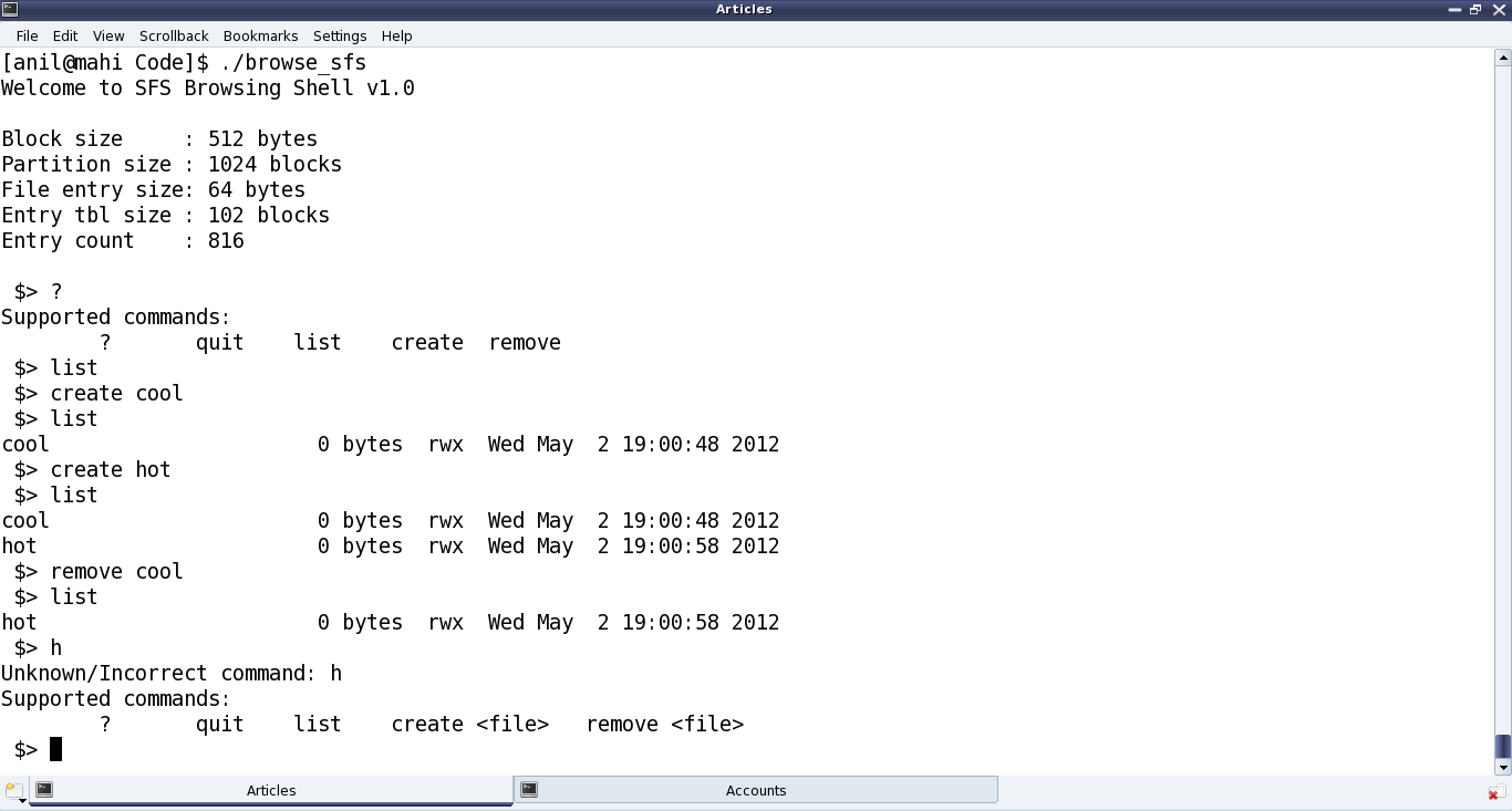
Figure 34: Simula file system browser output
sfs_list() traverses through all the file entries in the partition and prints all the non-null filename entries – with file name, size, permissions, and its creation time stamp. sfs_create() looks up for an available (null filename) entry and then updates it with the given filename, size of 0 bytes, permissions of “rwx”, and the current time stamp. And sfs_remove() looks up for an existing file entry, having the filename to be removed, and then nullifies it. The other parts in the above code are more of basic error handling cases like invalid command in browse_sfs(), existing file name in sfs_create(), non-existing file name in sfs_remove(), etc.
Note that the above application is the first-cut one of a full-fledged application. And so the files created right now are just with the basic fixed parameters. And, there is no way to change their permissions, content, etc, yet. However, it must be clear by now that adding those features is just a matter of adding commands and their corresponding functions, which would be provided for a few more interesting features by Shweta as she further works out the details of the browsing application.
Summing up
Once done with the other features as well, the next set of steps would take the project duo further closer to their final goals. Watch out for who takes charge of the next step of moving the file system logic to the kernel space.