This fourteenth article, which is part of the series on Linux device drivers, takes you for a walk inside a hard disk.
Hard disk design
“Doesn’t it sound like a mechanical engineering subject: Design of hard disk?”, questioned Shweta. “Yes, it does. But understanding it gets us an insight into its programming aspect”, reasoned Pugs while waiting for the commencement of the seminar on storage systems.
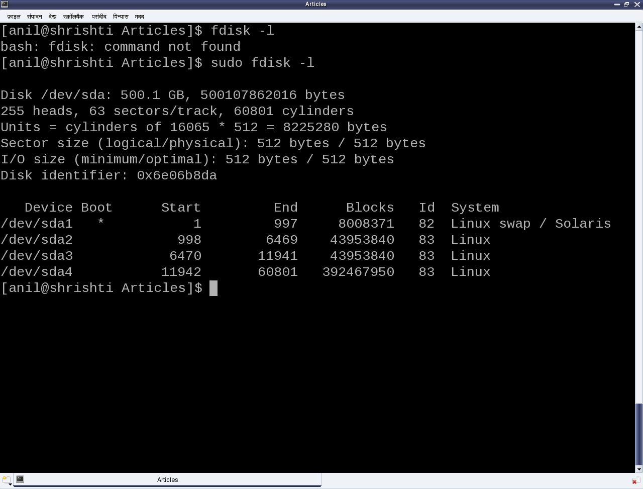
Figure 23: Partition listing by fdisk
The seminar started with a few hard disks in the presenter’s hand and then a dive down into her system showing the output of fdisk -l, as shown in Figure 23. The first line shows the hard disk size in human friendly format and in bytes. The second line mentions the number of logical heads, logical sectors per track, and the actual number of cylinders on the disk – these together are referred as the geometry of the disk. The 255 heads indicating the number of platters or disks, as one read-write head is needed per disk. Let’s number them say D1, D2, …, D255. Now, each disk would have the same number of concentric circular tracks, starting from outside to inside. In the above case there are 60801 such tracks per disk. Let’s number them say T1, T2, …, T60801. And a particular track number from all the disks forms a cylinder of the same number. For example, tracks T2 from D1, D2, …, D255 will all together form the cylinder C2. Now, each track has the same number of logical sectors – 63 in our case, say S1, S2, …, S63. And each sector is typically 512 bytes. Given this data, one can actually compute the total usable hard disk size, using the following formula:
Usable hard disk size in bytes = (Number of heads or disks) * (Number of tracks per disk) * (Number of sectors per track) * (Number of bytes per sector, i.e. sector size).
For the disk under consideration it would be: 255 * 60801 * 63 * 512 bytes = 500105249280 bytes. Note that this number may be slightly less than the actual hard disk – 500107862016 bytes in our case. The reason for that is that the formula doesn’t consider the bytes in last partial or incomplete cylinder. And the primary reason for that is the difference between today’s technology of organizing the actual physical disk geometry and the traditional geometry representation using heads, cylinders, sectors. Note that in the fdisk output, we referred to the heads, and sectors per track as logical not the actual one. One may ask, if today’s disks doesn’t have such physical geometry concepts, then why to still maintain that and represent them in more of logical form. The main reason is to be able to continue with same concepts of partitioning and be able to maintain the same partition table formats especially for the most prevalent DOS type partition tables, which heavily depend on this simplistic geometry. Note the computation of cylinder size (255 heads * 63 sectors / track * 512 bytes / sector = 8225280 bytes) in the third line and then the demarcation of partitions in units of complete cylinders.
DOS type partition tables
This brings us to the next important topic of understanding the DOS type partition tables. But in the first place, what is a partition and rather why to even partition? A hard disk can be divided into one more logical disks, each of which is called a partition. And this is useful for organizing different types of data separately. For example, different operating system data, user data, temporary data, etc. So, partitions are basically logical divisions and hence need to be maintained through some meta data, which is the partition table. A DOS type partition table contains 4 partition entries, each being a 16-byte entry. And each of these entries can be depicted by the following ‘C’ structure:
typedef struct
{
	unsigned char boot_type; // 0x00 - Inactive; 0x80 - Active (Bootable)
	unsigned char start_head;
	unsigned char start_sec:6;
	unsigned char start_cyl_hi:2;
	unsigned char start_cyl;
	unsigned char part_type;
	unsigned char end_head;
	unsigned char end_sec:6;
	unsigned char end_cyl_hi:2;
	unsigned char end_cyl;
	unsigned int abs_start_sec;
	unsigned int sec_in_part;
} PartEntry;
And this partition table followed by the two-byte signature 0xAA55 resides at the end of hard disk’s first sector, commonly known as Master Boot Record or MBR (in short). Hence, the starting offset of this partition table within the MBR is 512 – (4 * 16 + 2) = 446. Also, a 4-byte disk signature is placed at the offset 440. The remaining top 440 bytes of the MBR are typically used to place the first piece of boot code, that is loaded by the BIOS to boot up the system from the disk. Listing of part_info.c contains these various defines, and the code for parsing and printing a formatted output of the partition table of one’s hard disk.
From the partition table entry structure, it could be noted that the start and end cylinder fields are only 10 bits long, thus allowing a maximum of 1023 cylinders only. However, for today’s huge hard disks, this size is no way sufficient. And hence in overflow cases, the corresponding <head, cylinder, sector> triplet in the partition table entry is set to the maximum value, and the actual value is computed using the last two fields: the absolute start sector number (abs_start_sec) and the number of sectors in this partition (sec_in_part). Listing of part_info.c contains the code for this as well.
#include <stdio.h>
#include <sys/types.h>
#include <sys/stat.h>
#include <fcntl.h>
#include <unistd.h>

#define MBR_DISK_SIGNATURE_OFFSET 440
#define PARTITION_ENTRY_SIZE 16 // sizeof(PartEntry)
#define PARTITION_TABLE_SIZE (4 * PARTITION_ENTRY_SIZE)

typedef struct
{
	unsigned char boot_type; // 0x00 - Inactive; 0x80 - Active (Bootable)
	unsigned char start_head;
	unsigned char start_sec:6;
	unsigned char start_cyl_hi:2;
	unsigned char start_cyl;
	unsigned char part_type;
	unsigned char end_head;
	unsigned char end_sec:6;
	unsigned char end_cyl_hi:2;
	unsigned char end_cyl;
	unsigned int abs_start_sec;
	unsigned int sec_in_part;
} PartEntry;

typedef struct
{
	unsigned char boot_code[MBR_DISK_SIGNATURE_OFFSET];
	unsigned int disk_signature;
	unsigned short pad;
	unsigned char pt[PARTITION_TABLE_SIZE];
	unsigned short signature;
} MBR;

void print_computed(unsigned int sector)
{
	unsigned int heads, cyls, tracks, sectors;

	sectors = sector % 63 + 1 /* As indexed from 1 */;
	tracks = sector / 63;
	cyls = tracks / 255 + 1 /* As indexed from 1 */;
	heads = tracks % 255;
	printf("(%3d/%5d/%1d)", heads, cyls, sectors);
}

int main(int argc, char *argv[])
{
	char *dev_file = "/dev/sda";
	int fd, i, rd_val;
	MBR m;
	PartEntry *p = (PartEntry *)(m.pt);

	if (argc == 2)
	{
		dev_file = argv[1];
	}
	if ((fd = open(dev_file, O_RDONLY)) == -1)
	{
		fprintf(stderr, "Failed opening %s: ", dev_file);
		perror("");
		return 1;
	}
	if ((rd_val = read(fd, &m, sizeof(m))) != sizeof(m))
	{
		fprintf(stderr, "Failed reading %s: ", dev_file);
		perror("");
		close(fd);
		return 2;
	}
	close(fd);
	printf("\nDOS type Partition Table of %s:\n", dev_file);
	printf("  B Start (H/C/S)   End (H/C/S) Type  StartSec    TotSec\n");
	for (i = 0; i < 4; i++)
	{
		printf("%d:%d (%3d/%4d/%2d) (%3d/%4d/%2d)  %02X %10d %9d\n",
			i + 1, !!(p[i].boot_type & 0x80),
			p[i].start_head,
			1 + ((p[i].start_cyl_hi << 8) | p[i].start_cyl),
			p[i].start_sec,
			p[i].end_head,
			1 + ((p[i].end_cyl_hi << 8) | p[i].end_cyl),
			p[i].end_sec,
			p[i].part_type,
			p[i].abs_start_sec, p[i].sec_in_part);
	}
	printf("\nRe-computed Partition Table of %s:\n", dev_file);
	printf("  B Start (H/C/S)   End (H/C/S) Type  StartSec    TotSec\n");
	for (i = 0; i < 4; i++)
	{
		printf("%d:%d ", i + 1, !!(p[i].boot_type & 0x80));
		print_computed(p[i].abs_start_sec);
		printf(" ");
		print_computed(p[i].abs_start_sec + p[i].sec_in_part - 1);
		printf(" %02X %10d %9d\n", p[i].part_type,
			p[i].abs_start_sec, p[i].sec_in_part);
	}
	printf("\n");
	return 0;
}
As the above code (part_info.c) is an application, compile it to an executable (./part_info) as follows: gcc part_info.c -o part_info, and then run ./part_info /dev/sda to check out your primary partitioning information on /dev/sda. Figure 24 shows the output of ./part_info on the presenter’s system. Compare it with the fdisk output as shown in figure 23.
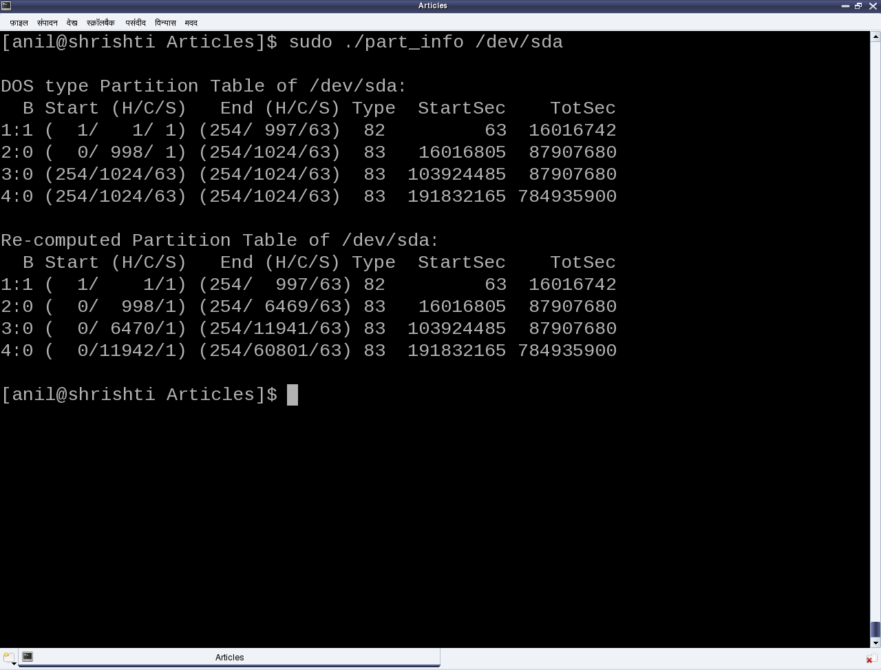
Figure 24: Output of ./part_info
Partition types and Boot records
Now as this partition table is hard-coded to have 4 entries, that dictates the maximum number of partitions, we can have, namely 4. These are called primary partitions, each having a type associated with them in their corresponding partition table entry. The various types are typically coined by the various operating system vendors and hence it is a sort of mapping to the various operating systems, for example, DOS, Minix, Linux, Solaris, BSD, FreeBSD, QNX, W95, Novell Netware, etc to be used for/with the particular operating system. However, this is more of ego and formality than a real requirement.
Apart from these, one of the 4 primary partitions can actually be labeled as something referred as an extended partition, and that has a special significance. As name suggests, it is used to further extend the hard disk division, i.e. to have more partitions. These more partitions are referred as logical partitions and are created within the extended partition. Meta data of the logical partitions is maintained in a linked list format, allowing unlimited number of logical partitions, at least theoretically. For that, the first sector of the extended partition, commonly referred to as Boot Record or BR (in short), is used in a similar way as MBR to store (the linked list head of) the partition table for the logical partitions. Subsequent linked list nodes are stored in the first sector of the subsequent logical partitions, referred to as Logical Boot Record or LBR (in short). Each linked list node is a complete 4-entry partition table, though only the first two entries are used – the first for the linked list data, namely, information about the immediate logical partition, and second one as the linked list’s next pointer, pointing to the list of remaining logical partitions.
To compare and understand the primary partitioning details on your system’s hard disk, follow these steps (as root user and hence with care):
- ./part_info /dev/sda # Displays the partition table on /dev/sda
- fdisk -l /dev/sda # To display and compare the partition table entries with the above
In case you have multiple hard disks (/dev/sdb, …), or hard disk device file with other names (/dev/hda, …), or an extended partition, you may try ./part_info <device_file_name> on them as well. Trying on an extended partition would give the information about the starting partition table of the logical partitions.
Summing up
“Right now we carefully and selectively played (read only) with our system’s hard disk. Why carefully? As otherwise, we may render our system non-bootable. But no learning is complete without a total exploration. Hence, in our post-lunch session, we would create a dummy disk on RAM and do the destructive explorations.”