This eleventh article of the mathematical journey through open source, explains curve fitting & interpolation with polynomials in octave.
In various fields of physics, chemistry, statistics, economics, … we very often come across something called curve fitting, and interpolation.
Given a set of data points from our observations, we would like to see what mathematical equation does they follow. So, we try to fit the best curve through those data points, called the curve fitting technique. Once we have the equation, the main advantage is that then we can find the values at the points, we haven’t observed by just substituting that value in the equation. One may think of this as interpolation. But this is not exactly interpolation. As in interpolation, we are restricted to finding unobserved values only between two observed points, using a pre-defined curve fit between those two points. With that we may not be able to get values outside our observation range. But the main reason for using that is when we are not interested or it is not meaningful or we are unable to fit a known form of curve in the overall data set, but still we want to get some approximations of values, in between the observed data points. Enough of gyaan, now let’s look into each one of those.
Curve Fitting
Let’s say for any system, we have the following data points:
For the inputs of 1, 3, 6, 10, 20, we get the outputs as 2.5, 7.5, 15.5, 24, 45, respectively. Then, we would like to know as how is input is related to the output. So, to get a feel of the relation, we first plot this points on a x-y plane, say inputs as x and outputs as y. Figure 6 shows the same. And the octave code for that is as follows:
$ octave -qf
octave:1> x = [1 3 6 10 20];
octave:2> y = [2.5 7.5 15.5 24 45];
octave:3> plot(x, y, "*");
octave:4> xlabel("Inputs");
octave:5> ylabel("Outputs");
octave:6>
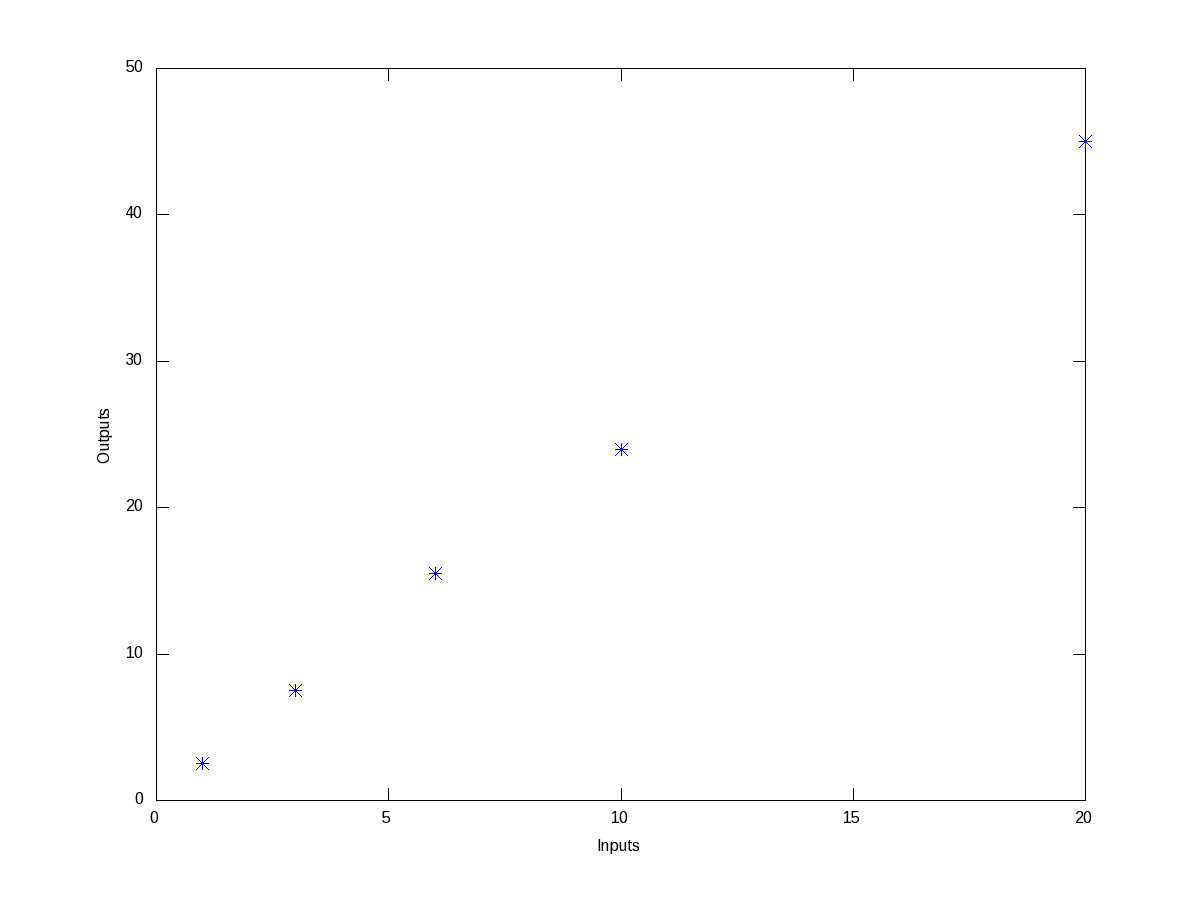
Figure 6: Plot of the data points
By observing the plot, the simplest fitting relation looks to be a straight line. So, let’s try fitting a linear polynomial, i.e. a first order polynomial, i.e. a straight line. Here’s the code in execution for it:
octave:1> x = [1 3 6 10 20];
octave:2> y = [2.5 7.5 15.5 24 45];
octave:3> p = polyfit(x, y, 1)
p =

   2.2212   1.1301

octave:4> polyout(p, "x");

2.2212*x^1 + 1.1301

octave:5> plot(x, y, "*", x, polyval(p, x), "-");
octave:6> xlabel("Inputs");
octave:7> ylabel("Outputs");
octave:8> legend("Data points", "Linear Fit");
octave:9>
polyfit() takes 3 arguments, the x values, the y values, and the order of the polynomial to fit – 1 for linear. It then returns the coefficients of the fitted polynomial p. polyout() displays the polynomial in more readable format. So, the fitted equation is y = 2.2212 * x + 1.1301. polyval() takes the polynomial p and the input values x, and calculates the output values y, as per the polynomial equation. And then we plot them, along with the earlier data points, on the same plot. Figure 7 shows the same, 2.2212 being the slope / gradient of the straight line, and 1.1301 being the intercept. Now, we notice that the straight line does not fit exactly, and there is some deviation from the observed points. polyfit() fits the polynomial with the minimum deviation for the order we request, but still there is a deviation, as that is the minimum possible. If you want to get the standard deviation for the particular fit, you just need to do the following:
octave:9> std_dev = sqrt(mean((y - polyval(p, x)).^2))
std_dev =  0.72637
octave:10>

Figure 7: Linear fit of data points
And we see that it is a small value compared to our output values. But say we are not fully satisfied with this, we may like to try higher order polynomials, say of order 2, a quadratic, and observe the results from it. Here’s how one would do this:
octave:1> x = [1 3 6 10 20];
octave:2> y = [2.5 7.5 15.5 24 45];
octave:3> p = polyfit(x, y, 2)
p =

  -0.018639   2.623382  -0.051663

octave:4> polyout(p, "x");

-0.018639*x^2 + 2.6234*x^1 - 0.051663

octave:5> plot(x, y, "*", x, polyval(p, x), "-");
octave:6> xlabel("Inputs");
octave:7> ylabel("Outputs");
octave:8> legend("Data points", "Quadratic Fit");
octave:9> std_dev = sqrt(mean((y - polyval(p, x)).^2))
std_dev =  0.26873
octave:10>
Figure 8 shows the data points and fitted quadratic curve. All the values above can be interpreted in the similar way as earlier. And we note that the standard deviation has come down further. In fact, as we increase the polynomial order further and further, we will definitely note that the standard deviation keeps on decreasing, till the order is same as number of data points – 1, after which it remains 0. But, we may not like to do this, as our observed data points are typically not perfect, and we are typically not interested in getting the standard deviation zero but for a fit more appropriate to reflect the relation between the system’s input and output.
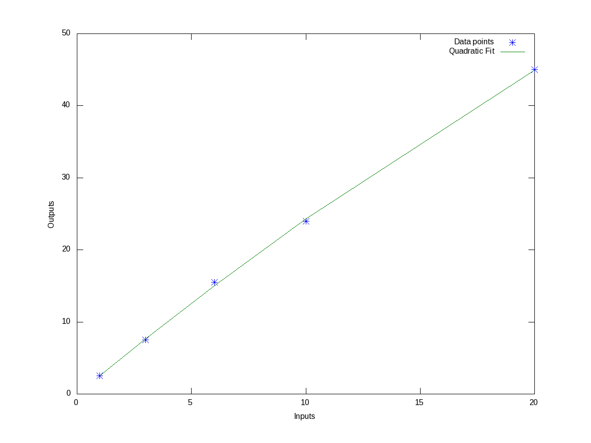
Figure 8: Quadratic fit of data points
Interpolation
Now, say we have the following wierd data points, listed as (x, y) pairs: (1, 1), (2, 2), (3, 3), (4, 2), (5, 1), (6, 3.75), (7, 7), (8, 3), (9, 0), (11, 8). Figure 9 shows, how wierd they look like.
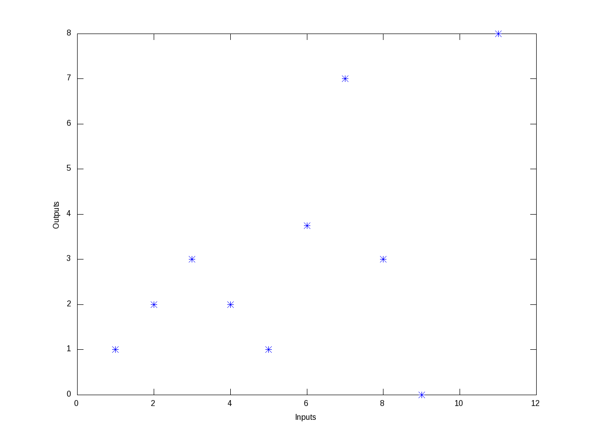
Figure 9: Wierd data points
Trying to fit a polynomial, would be quite meaningless. But still they seem to have some correlation in between smaller ranges of input, say between 1 and 3, 3 and 5, 5 and 7, and so on. So, this is best suited for us to do interpolation for finding the values in between, say at 1.5, 3.8, 10, … Now interpolation is all about curve fitting between two neighbouring data points and then calculating the value at any intermediate point. So, the typical varieties of techniques used for this “piece-wise curve fitting” are:
- nearest: Return the nearest data point (actually no curve fitting)
- linear: Linear/Straight line fitting between the two neighbouring data points
- pchip: Piece-wise cubic (order 3) hermite polynomial fitting
- cubic: Cubic (order 3) polynomial fitted between four nearest neighbouring data points
- spline: Cubic (order 3) spline fitting with smooth first and second derivatives throughout the curve
All these may look little jargonish – so don’t worry about that. Let’s just try out some examples to drive the point home. Here’s the code to show the nearest & linear interpolation for the above data:
octave:1> x = [1 2 3 4 5 6 7 8 9 11];
octave:2> y = [1 2 3 2 1 3.75 7 3 0 8];
octave:3> xi = 1:0.1:11;
octave:4> y_n = interp1(x, y, xi, "nearest");
octave:5> y_l = interp1(x, y, xi, "linear");
octave:6> plot(x, y, "*", xi, y_n, "-", xi, y_l, "-");
octave:7> xlabel("Inputs");
octave:8> ylabel("Outputs");
octave:9> legend("Data points", "Nearest", "Linear");
octave:10>
Figure 10 shows the same.
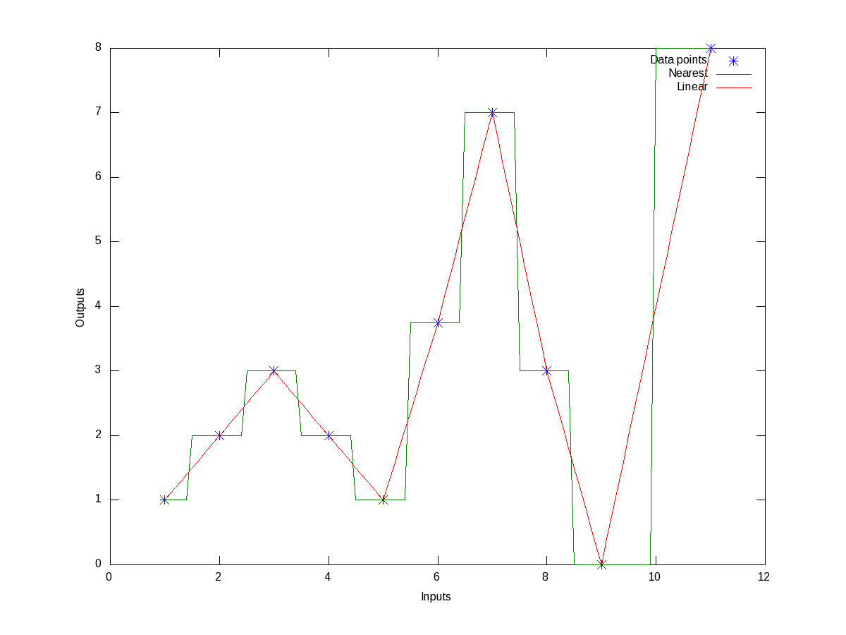
Figure 10: Nearest and linear interpolations of the data points
Now, if we want to get the interpolated values say at the points 1.5, 3.8, 10, instead of giving all the intermediate points xi in the above code, we may just give these 3 – that’s all. Here goes the code in execution for the that:
octave:1> x = [1 2 3 4 5 6 7 8 9 11];
octave:2> y = [1 2 3 2 1 3.75 7 3 0 8];
octave:3> our_x = [1.5 3.8 10];
octave:4> our_y_n = interp1(x, y, our_x, "nearest")
our_y_n =

   2   2   8

octave:5> our_y_l = interp1(x, y, our_x, "linear")
our_y_l =

   1.5000   2.2000   4.0000

octave:6>
Now, before closing on interpolation, just to give a feel of all of the interpolation techniques, here goes an example with the points on a sine curve:
octave:1> x = 0:2*pi;
octave:2> y = sin(x);
octave:3> xi = 0:0.1:2*pi;
octave:4> y_n = interp1(x, y, xi, "nearest");
octave:5> y_l = interp1(x, y, xi, "linear");
octave:6> y_p = interp1(x, y, xi, "pchip");
octave:7> y_c = interp1(x, y, xi, "cubic");
octave:8> y_s = interp1(x, y, xi, "spline");
octave:9> plot(x, y, "*", xi, y_n, "-", xi, y_l, "-", xi, y_p, "-", xi, y_c, "-",
                                                                      xi, y_s, "-");
octave:10> xlabel("x ->");
octave:11> ylabel("y ->");
octave:12> legend("Data points", "Nearest", "Linear", "Pchip", "Cubic", "Spline");
octave:13> print("-dpng", "all_types_of_interpolations.png");
octave:14>
Figure 11 shows the visualization of the same for your eyes.
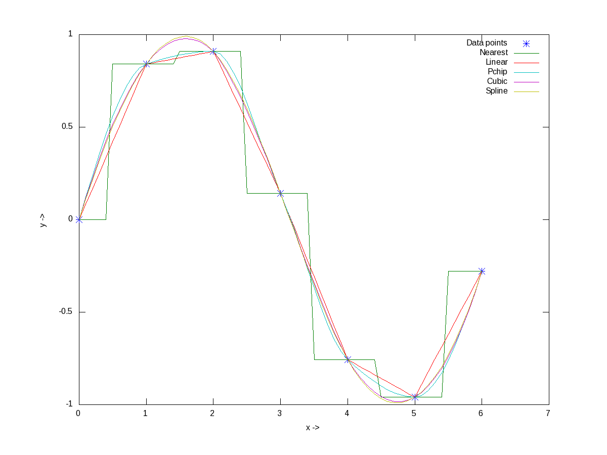
Figure 11: All types of interpolations for sinusoidal points
What’s next?
With today’s curve fitting & interpolation walk through, we have used some basic 2-D plotting techniques. But there are many more features and techniques to plotting, like marking our plots, visualizing 3-D stuff, etc. Next, we’ll look into that.
The author is a hobbyist in open source hardware and software, with a passion for mathematics, and philosopher in thoughts. A gold medallist from the Indian Institute of Science, Linux, mathematics and knowledge sharing are few of his passions. He experiments with Linux and embedded systems to share his learnings through his weekend workshops. Learn more about him and his experiments at https://sysplay.in.


Pingback: Polynomial Power of Octave | Playing with Systems
Pingback: Figures, Graphs, and Plots in Octave | Playing with Systems