Tag Archives: Matrices

Solve Non-linear Equations using Linear Algebra

This eighth article of the mathematical journey through open source, solves non-linear equations using linear algebra in octave.

<< Seventh Article

Hope you have found out the vegetable prices from the vegetable seller, who had placed various equal priced stacks for sell at ₹30. Recall: One stack had 4 lemons, 7 cucumbers, 9 tomatoes. Another had 2 lemons, 5 cucumbers, 27 tomatoes. And the third had just 9 cucumbers & 15 tomatoes. Prices would be ₹2.00 per lemon, ₹2.50 per cucumber, ₹0.50 per tomato, computed as follows:

$ octave -qf
octave:1> N = [
> 4 7 9
> 2 5 27
> 0 9 15
> ];
octave:2> inv(N) * [30; 30; 30]
ans =

   2.00000
   2.50000
   0.50000

octave:3>

Polynomial solving

Note that though in 3 variables, even this was a linear equation. How about solving higher order polynomial equations, meaning of squares, cubes, … of the variables. Say, we want a solution for x in x3 + 3x2 + 3x + 1 = 0. Simple! First define a function for this polynomial. And, then use the function solver fsolve() to solve it, as follows:

$ octave -qf
octave:1> function y = f(x)
> y = x^3 + 3*x^2 + 3*x + 1;
> endfunction
octave:2> [x, fval, info] = fsolve(@f, 0)
x = -0.99999
fval = 0
info =  1
octave:3>

This indicates the value of x as -0.99999 ≈ -1 as the solution to the function f(x), yielding a function value of 0, with info = 1 indicating that solution is obtained. And you may verify the answer by calling the function f with the variable x as f(x) on the octave prompt. The second parameter in fsolve() is the initial guess of the solution.

Geometry solving

With the power in hand, why not solve more complex geometric problems? Last time we found the intersection point of two straight lines. How about intersection of a straight line and a circle? Let us have the following straight line and circle, defined in the Cartesian coordinate system, i.e. the x-y system:
4x + 3y = 24
x2 + y2 = 25

To be able to solve it using fsolve(), let’s consider the different variables x & y as fields of a vector X, say x as X(1), y as X(2). Then, the equations can be re-written as follows:
4 * X(1) + 3 * X(2) = 24
X(1)^2 + X(2)^2 = 25
and hence could be solved using fsolve() as follows:

$ octave -qf
octave:1> function Y = F(X)
> Y(1) = 4 * X(1) + 3 * X(2) - 24;
> Y(2) = X(1)^2 + X(2)^2 - 25;
> endfunction
octave:2> [Y, Fval, info] = fsolve(@F, [0; 0])
warning: matrix singular to machine precision, rcond = 0
warning: attempting to find minimum norm solution
warning: dgelsd: rank deficient 2x2 matrix, rank = 1
Y =

   3.0000
   4.0000

Fval =

   0.0000e+00   2.6691e-07

info =  1
octave:3>

So, (3, 4) is the intersecting point – can be verified by substituting back into the above equations.

Solve it

Equipped with this knowledge, here’s a couple of teasers for your brain:

  1. Find three numbers, product of which is 60; sum of their squares is 50; and their sum is 12.
  2. A sage came to a temple with some flowers and dipped all of them into the first magical pond of the temple and got those back, squared. Then, he offered some of those flowers in the temple and dipped the remaining flowers into the second magical pond to get those back, doubled. Then, he again offered the same number of flowers, as offered earlier, and dipped the remaining flowers into the third magical pond to get those back, tripled, which he took back with him as prasadam. Now, the number of flowers he took back with him, is same as in each one of his offerings. Also, what he took back with him is thrice the number of flowers he came with to the temple. How many flowers did he come in with?

If you think, you have got the octave code for solving the above, you may post the solution in the comments below. And as we move on, we would get into specifically playing with polynomials.
Ninth Article >>

   Send article as PDF   

Solve Puzzles using Linear Algebra

This seventh article of the mathematical journey through open source, solves puzzles using linear algebra in octave.

<< Sixth Article

Matrix Maths is what is formally called Linear Algebra. We have gone through its basics in the fifth article. Now, we shall apply that to practical usage. What better than solving puzzles using the same.

Purchase Solving

Shrishti purchased 24 pencils and 12 erasers for ₹96. Divya purchased 20 pencils and 15 erasers for ₹100. What are the prices of the pencil & the eraser?

Assuming that ‘p’ is the price for pencils & ‘e’ is the price for erasers, we have the following two equations:
24 * p + 12 * e = 96
20 * p + 15 * e = 100
Hence, we could get the values of ‘p’ & ‘e’ by solving these equations. Converting them into linear algebra form, they can be re-written using matrix multiplication as:
┏          ┓┏    ┓    ┏        ┓
┃24 12 ┃┃ p ┃    ┃   96 ┃
┃20 15 ┃┃ e ┃ = ┃ 100 ┃
┗          ┛┗    ┛    ┗        ┛
which is Ax = b, ‘x’ being the vector with variables ‘p’ & ‘e’. Hence, we need to solve for x, which is given by: x = A-1b. Using octave:

$ octave -qf
octave:1> A = [
> 24 12
> 20 15
> ];
octave:2> b = [
> 96
> 100
> ];
octave:3> x = inv(A) * b
x =

   2.0000
   4.0000

octave:4>

Hence, p = ₹2 and e = ₹4, i.e. each pencil costs ₹2 and an eraser costs ₹4. You may check by putting back these values in our problem statement. Isn’t that cool?

Geometry Solving

How about finding the intersection point of two straight lines? Let us have the following 2 straight lines, defined in the Cartesian coordinate system, i.e. the x-y system:
4x + 3y = 24
3x + 4y = 25

Similar to the earlier problem, the intersecting point could be obtained as follows:

$ octave -qf
octave:1> A = [
> 4 3
> 3 4
> ];
octave:2> b = [
> 24
> 25
> ];
octave:3> X = inv(A) * b
X =

   3.0000
   4.0000

octave:4>

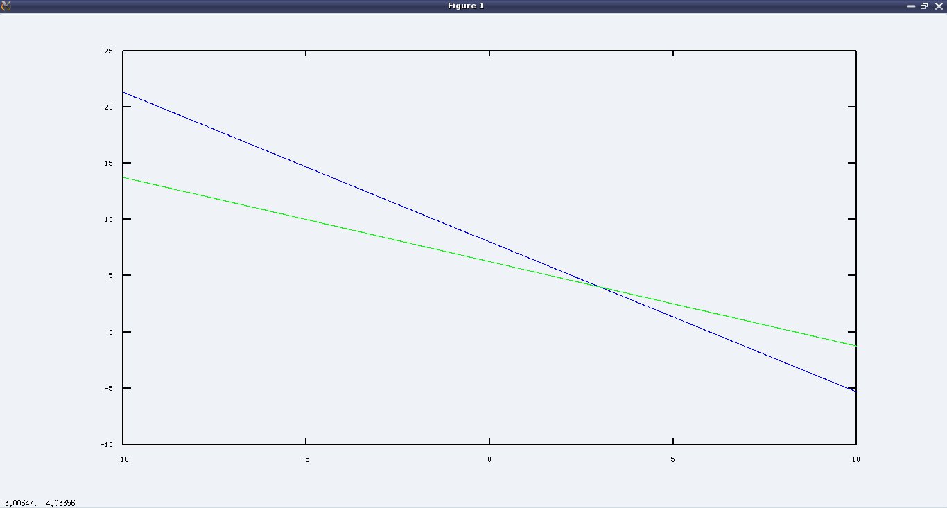
So, (3, 4) is the intersecting point. Want to see it visually. For that, we would just need to rewrite the straight line equations as follows:
y = (24 – 4x) / 3
y = (25 – 3x) / 4
And then here goes the code:

octave:1> x=-10:0.01:10;
octave:2> plot(x, (24 - 4*x)/3, "b.", x, (25 - 3*x)/4, "g.");
octave:3>

Figure 5 shows the plot generated by the above code.

Figure 5: Intersection of straight lines

Figure 5: Intersection of straight lines

Solve it

Equipped with the puzzle solving basics, here’s one for your brain: A vegetable seller has placed various equal priced stacks for sale at ₹30. One stack has 4 lemons, 7 cucumbers, 9 tomatoes. Another has 2 lemons, 5 cucumbers, 27 tomatoes. And the third has just 9 cucumbers & 15 tomatoes. Can you compute the price of each vegetable?

Hint: Assume the price of lemon, cucumber, tomato as ‘l’, ‘c’, ‘t’, and then form the 3 equations in three variables.

If you think, you have got it, you may post the solution in the comments. And as we move on, we will get into some different kind of puzzle solving.

Eighth Article >>

   Send article as PDF   

Mathematics made easy with minimal Octave

This fifth article of the mathematical journey through open source, introduces the minimal, octave can do for you.

<< Fourth Article

You wanted a non-programmers way of doing mathematics and there you go – octave. Sounds like something to do with music, but in reality it is the name the octave author’s chemical engineering professor, who was well know for his ‘back of the envelope’ calculations.

All of bench calculator!!!

All the operations of bench calculator are just a subset of octave. So, no point going round the wheel again. Whatever operations can be done in bc – arithmetic, logical, relational, conditional – all can be done with equal ease in octave. As in bc, it can as well be used as a mathematical programming language. Ha! Then, why did we waste time on learning bc, we could have straight away come to octave. Yes! Yes! Except one thing – the precision-less-ness. We can’t get that in octave. If we need that, we would have to go back to bc. Okay! Fine. So, what with octave – we start with N-dimensions, what else. Hey don’t worry! In simple language, I mean vectors & matrices.

Getting Started

Command: Typing ‘octave‘ on the shell brings up the octave‘s interactive shell. Type ‘quit’ or Control-D to exit. The interactive shell starts with a welcome message. As in bc, we pass option -q for it to not show. Additionally, we’ll use the -f option for it to not pick any local start-up scripts (if any). So, for our examples, the command would look like ‘octave -qf‘ to start octave with an interactive shell.

Prompts & Results: Input prompt is typically denoted by ‘octave:X>‘, where X just a number showing the command count. Valid results are typically shown with ‘<variable> = ‘, or ‘ans = ‘ or ‘=> ‘, and then the command count incremented for the next input. Errors cause error messages to be printed and then octave brings back the input prompt without incrementing the command count. Putting a semicolon (;) at the end of an statement, suppresses it result (return value) to be displayed.

Comments could start with # or %. For block comments, #{ … }# or %{ … }% can be used.

Detailed topic help could be obtained using ‘help <topic>’ or complete documentation using ‘doc’ on the octave shell.

All in a go:

$ octave -qf
octave:1> # This is a comment
octave:1> pi # Built-in constant
ans =  3.1416
octave:2> e # Built-in constant again
ans =  2.7183
octave:3> i # Same as j – the imaginary number
ans =  0 + 1i
octave:4> x = 3^4 + 2*30;
octave:5> x
x =  141
octave:6> y
error: `y' undefined near line 6 column 1
octave:6> doc # Complete doc; Press 'q' to come back
octave:7> help plot # Help on plot
octave:8> A = [1 2 3; 4 5 6; 7 8 9] # 3x3 matrix
A =

   1   2   3
   4   5   6
   7   8   9

octave:9> quit

Matrices with a Heart

Yes, we already saw a matrix in creation. It can also be created through multiple lines. Octave continues waiting for further input by prompting just ‘>’. Checkout below for creating the 3×3 magic square matrix in the same way, followed by various other interesting operations:

$ octave -qf
octave:1> M = [ # 3x3 magic square
> 8 1 6
> 3 5 7
> 4 9 2
> ]
M =

   8   1   6
   3   5   7
   4   9   2

octave:2> B = rand(3, 4); # 3x4 matrix w/ randoms in [0 1]
octave:3> B
B =

   0.068885   0.885998   0.542059   0.797678
   0.652617   0.904360   0.036035   0.737404
   0.043852   0.579838   0.709194   0.053118

octave:4> B' # Transpose of B
ans =

   0.068885   0.652617   0.043852
   0.885998   0.904360   0.579838
   0.542059   0.036035   0.709194
   0.797678   0.737404   0.053118

octave:5> A = inv(M) # Inverse of M
A =

   0.147222  -0.144444   0.063889
  -0.061111   0.022222   0.105556
  -0.019444   0.188889  -0.102778

octave:6> M * A # Should be identity, at least approx.
ans =

   1.00000   0.00000  -0.00000
  -0.00000   1.00000   0.00000
   0.00000   0.00000   1.00000

octave:7> function rv = psine(x) # Our phase shifted sine
>
> rv = sin(x + pi / 6);
>
>  endfunction 
octave:8> x = linspace(0, 2*pi, 400); # 400 pts from 0 to 2*pi
octave:9> plot(x, psine(x)) # Our function's plot
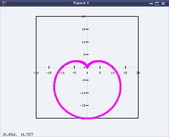
octave:10> polar(x, 10 * (1 - sin(x)), 'm*') # bonus Heart
octave:11> quit

Figure 1 shows the plot window which pops up by the command # 9 – plot.

Figure 2 is the bonus magenta heart of stars (*) from polar coordinates draw command # 10 – polar.

Figure 1: Plot of our 30° phase shifted sine

Figure 1: Plot of our 30° phase shifted sine

Figure 2: The Heart

Figure 2: The Heart

What next?

With ready-to-go level of introduction to octave, we are all set to explore it the fun way. What fun? Next one left to your imagination. And as we move on, we would take up one or more fun challenge(s), and try to see, how we solve it using octave.

Sixth Article >>

   Send article as PDF