Tag Archives: OSFY

File Systems: The Semester Project – Part II

This nineteenth article, which is part of the series on Linux device drivers, continues with introducing the concept of a file system, by simulating one in user space.

<< Eighteenth Article

In the previous article, Shweta readied the partition on the .sfsf file by formating it with the format_sfs application. To complete the understanding of a file system, the next step in its simulation is to browse and play around with the file system created. Here is Shweta’s first-cut browser application to achieve the same. Let’s have a closer look. sfs_ds.h is the same header file, already created by Shweta.

#include <stdio.h>
#include <sys/types.h>
#include <sys/stat.h>
#include <fcntl.h>
#include <unistd.h>
#include <string.h>
#include <time.h>

#include "sfs_ds.h"

sfs_super_block_t sb;

void sfs_list(int sfs_handle)
{
	int i;
	sfs_file_entry_t fe;

	lseek(sfs_handle, sb.entry_table_block_start * sb.block_size, SEEK_SET);
	for (i = 0; i < sb.entry_count; i++)
	{
		read(sfs_handle, &fe, sizeof(sfs_file_entry_t));
		if (!fe.name[0]) continue;
		printf("%-15s  %10d bytes  %c%c%c  %s",
			fe.name, fe.size,
			fe.perms & 04 ? 'r' : '-',
			fe.perms & 02 ? 'w' : '-',
			fe.perms & 01 ? 'x' : '-',
			ctime((time_t *)&fe.timestamp)
			);
	}
}
void sfs_create(int sfs_handle, char *fn)
{
	int i;
	sfs_file_entry_t fe;

	lseek(sfs_handle, sb.entry_table_block_start * sb.block_size, SEEK_SET);
	for (i = 0; i < sb.entry_count; i++)
	{
		read(sfs_handle, &fe, sizeof(sfs_file_entry_t));
		if (!fe.name[0]) break;
		if (strcmp(fe.name, fn) == 0)
		{
			printf("File %s already exists\n", fn);
			return;
		}
	}
	if (i == sb.entry_count)
	{
		printf("No entries left\n", fn);
		return;
	}

	lseek(sfs_handle, -(off_t)(sb.entry_size), SEEK_CUR);

	strncpy(fe.name, fn, 15);
	fe.name[15] = 0;
	fe.size = 0;
	fe.timestamp = time(NULL);
	fe.perms = 07;
	for (i = 0; i < SIMULA_FS_DATA_BLOCK_CNT; i++)
	{
		fe.blocks[i] = 0;
	}

	write(sfs_handle, &fe, sizeof(sfs_file_entry_t));
}
void sfs_remove(int sfs_handle, char *fn)
{
	int i;
	sfs_file_entry_t fe;

	lseek(sfs_handle, sb.entry_table_block_start * sb.block_size, SEEK_SET);
	for (i = 0; i < sb.entry_count; i++)
	{
		read(sfs_handle, &fe, sizeof(sfs_file_entry_t));
		if (!fe.name[0]) continue;
		if (strcmp(fe.name, fn) == 0) break;
	}
	if (i == sb.entry_count)
	{
		printf("File %s doesn't exist\n", fn);
		return;
	}

	lseek(sfs_handle, -(off_t)(sb.entry_size), SEEK_CUR);

	memset(&fe, 0, sizeof(sfs_file_entry_t));
	write(sfs_handle, &fe, sizeof(sfs_file_entry_t));
}

void browse_sfs(int sfs_handle)
{
	int done;
	char cmd[256], *fn;
	int ret;

	done = 0;

	printf("Welcome to SFS Browsing Shell v1.0\n\n");
	printf("Block size	 : %d bytes\n", sb.block_size);
	printf("Partition size : %d blocks\n", sb.partition_size);
	printf("File entry size: %d bytes\n", sb.entry_size);
	printf("Entry tbl size : %d blocks\n", sb.entry_table_size);
	printf("Entry count	: %d\n", sb.entry_count);
	printf("\n");
	while (!done)
	{
		printf(" $> ");
		ret = scanf("%[^\n]", cmd);
		if (ret < 0)
		{
			done = 1;
			printf("\n");
			continue;
		}
		else
		{
			getchar();
			if (ret == 0) continue;
		}
		if (strcmp(cmd, "?") == 0)
		{
			printf("Supported commands:\n");
			printf("\t?\tquit\tlist\tcreate\tremove\n");
			continue;
		}
		else if (strcmp(cmd, "quit") == 0)
		{
			done = 1;
			continue;
		}
		else if (strcmp(cmd, "list") == 0)
		{
			sfs_list(sfs_handle);
			continue;
		}
		else if (strncmp(cmd, "create", 6) == 0)
		{
			if (cmd[6] == ' ')
			{
				fn = cmd + 7;
				while (*fn == ' ') fn++;
				if (*fn != '')
				{
					sfs_create(sfs_handle, fn);
					continue;
				}
			}
		}
		else if (strncmp(cmd, "remove", 6) == 0)
		{
			if (cmd[6] == ' ')
			{
				fn = cmd + 7;
				while (*fn == ' ') fn++;
				if (*fn != '')
				{
					sfs_remove(sfs_handle, fn);
					continue;
				}
			}
		}
		printf("Unknown/Incorrect command: %s\n", cmd);
		printf("Supported commands:\n");
		printf("\t?\tquit\tlist\tcreate <file>\tremove <file>\n");
	}
}

int main(int argc, char *argv[])
{
	char *sfs_file = SIMULA_DEFAULT_FILE;
	int sfs_handle;

	if (argc > 2)
	{
		fprintf(stderr, "Incorrect invocation. Possibilities are:\n");
		fprintf(stderr,
			"\t%s /* Picks up %s as the default partition_file */\n",
			argv[0], SIMULA_DEFAULT_FILE);
		fprintf(stderr, "\t%s [ partition_file ]\n", argv[0]);
		return 1;
	}
	if (argc == 2)
	{
		sfs_file = argv[1];
	}
	sfs_handle = open(sfs_file, O_RDWR);
	if (sfs_handle == -1)
	{
		fprintf(stderr, "Unable to browse SFS over %s\n", sfs_file);
		return 2;
	}
	read(sfs_handle, &sb, sizeof(sfs_super_block_t));
	if (sb.type != SIMULA_FS_TYPE)
	{
		fprintf(stderr, "Invalid SFS detected. Giving up.\n");
		close(sfs_handle);
		return 3;
	}
	browse_sfs(sfs_handle);
	close(sfs_handle);
	return 0;
}

The above (shell like) program primarily reads the super block from the partition file (.sfsf by default, or the file provided from command line), and then gets into browsing the file system based on that information, using the browse_sfs() function. Note the check performed for the valid file system on the partition file using the magic number SIMULA_FS_TYPE.

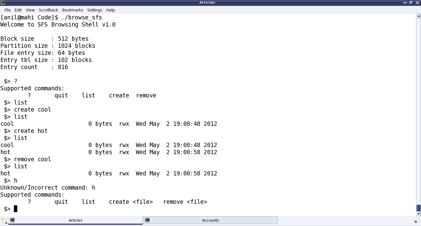
browse_sfs() prints the file system information and provides four basic file system functionalities using the following commands:

  • quit – to quit the file system browser
  • list – to list the current files in the file system (using sfs_list())
  • create <filename> – to create a new file in the file system (using sfs_create(filename))
  • remove <filename> – to remove an existing file from the file system (using sfs_remove(filename))

Figure 34 shows the browser in action, using the above commands.

Figure 34: Simula file system browser output

Figure 34: Simula file system browser output

sfs_list() traverses through all the file entries in the partition and prints all the non-null filename entries – with file name, size, permissions, and its creation time stamp. sfs_create() looks up for an available (null filename) entry and then updates it with the given filename, size of 0 bytes, permissions of “rwx”, and the current time stamp. And sfs_remove() looks up for an existing file entry, having the filename to be removed, and then nullifies it. The other parts in the above code are more of basic error handling cases like invalid command in browse_sfs(), existing file name in sfs_create(), non-existing file name in sfs_remove(), etc.

Note that the above application is the first-cut one of a full-fledged application. And so the files created right now are just with the basic fixed parameters. And, there is no way to change their permissions, content, etc, yet. However, it must be clear by now that adding those features is just a matter of adding commands and their corresponding functions, which would be provided for a few more interesting features by Shweta as she further works out the details of the browsing application.

Summing up

Once done with the other features as well, the next set of steps would take the project duo further closer to their final goals. Watch out for who takes charge of the next step of moving the file system logic to the kernel space.
Twentieth Article >>

   Send article as PDF   

Advanced Set Theory

This nineteenth article of the mathematical journey through open source, explores the advanced set theory concepts through Maxima.

<< Eighteenth Article

With the introduction to set theory fundamentals in the previous article, we are all set to explore the advanced realms of set theory through Maxima.

More set operations

We have already worked out the basic set creation techniques and some basic set operations provided by Maxima. Here are some next-level ones provided by Maxima:

  • makeset(expr, vars, varslist) – Sophisticated set creation using expressions
  • adjoin(x, S) – Returns a set with all elements of S and the element x
  • disjoin(x, S) – Returns a set with all elements S but without element x
  • powerset(S) – Returns the set of all subsets of S
  • subset(S, p) – Returns the subset of S, elements of which satisfy the predicate p
  • symmdifference(S1, S2) – Returns the symmetric difference between the sets S1 and S2, i.e. the elements in S1 or S2 but not in both

And here goes a demonstration of each one of them:

$ maxima -q
(%i1) makeset(a+b, [a, b], [[1, 2], [2, 3], [3, 4], [4, 5], [5, 6]]);
(%o1)                          {3, 5, 7, 9, 11}
(%i2) makeset(a-b, [a, b], [[1, 2], [2, 3], [3, 4], [4, 5], [5, 6]]);
(%o2)                                {- 1}
(%i3) makeset(a*b, [a, b], [[1, 2], [2, 3], [3, 4], [4, 5], [5, 6]]);
(%o3)                         {2, 6, 12, 20, 30}
(%i4) makeset(a + 2*a*b + b, [a, b], [[1, 2], [2, 3], [3, 4], [4, 5], [5, 6]]);
(%o4)                         {7, 17, 31, 49, 71}
(%i5) quit();
$ maxima -q
(%i1) S: {-4, 6, 7, 32, 0};
(%o1)                         {- 4, 0, 6, 7, 32}
(%i2) adjoin(3, S);
(%o2)                        {- 4, 0, 3, 6, 7, 32}
(%i3) adjoin(7, S);
(%o3)                        {- 4, 0, 6, 7, 32}
(%i4) S: adjoin(3, S); /* Updating S */
(%o4)                       {- 4, 0, 3, 6, 7, 32}
(%i5) adjoin(7, S);
(%o5)                       {- 4, 0, 3, 6, 7, 32}
(%i6) disjoin(7, S);
(%o6)                        {- 4, 0, 3, 6, 32}
(%i7) disjoin(5, S);
(%o7)                       {- 4, 0, 3, 6, 7, 32}
(%i8) quit();
$ maxima -q
(%i1) S: {-4, 0, 3, 6, 7, 32};
(%o1)                        {- 4, 0, 3, 6, 7, 32}
(%i2) S1: subset(S, evenp);
(%o2)                           {- 4, 0, 6, 32}
(%i3) powerset(S1);
(%o3) {{}, {- 4}, {- 4, 0}, {- 4, 0, 6}, {- 4, 0, 6, 32}, {- 4, 0, 32}, {- 4, 6},
	{- 4, 6, 32}, {- 4, 32}, {0}, {0, 6}, {0, 6, 32}, {0, 32}, {6}, {6, 32},
	{32}}
(%i4) S2: {-35, -26, 0, 7, 32, 100};
(%o4)                     {- 35, - 26, 0, 7, 32, 100}
(%i5) symmdifference(S1, S2);
(%o5)                    {- 35, - 26, - 4, 6, 7, 100}
(%i6) symmdifference(S, S2);
(%o6)                    {- 35, - 26, - 4, 3, 6, 100}
(%i7) quit();

Advanced set operations

With Maxima, much more than this can be done with sets, just by the functionalities provided by it. So now, let’s journey through such interesting advance functionalities:

Cartesian Product:

Given n sets, the function cartesian_product() returns a set of lists formed by the Cartesian product of the n sets. The following demonstration explains what it means:

$ maxima -q
(%i1) cartesian_product({0, 1, 2}, {a, b, c});
(%o1) {[0, a], [0, b], [0, c], [1, a], [1, b], [1, c], [2, a], [2, b], [2, c]}
(%i2) cartesian_product({0, 1}, {a, b}, {X, Y});
(%o2) {[0, a, X], [0, a, Y], [0, b, X], [0, b, Y], [1, a, X], [1, a, Y], [1, b, X],
	[1, b, Y]}
(%i3) cartesian_product({0, 1}, {a, b, c});
(%o3)          {[0, a], [0, b], [0, c], [1, a], [1, b], [1, c]}
(%i4) quit();

Set Partitions:

Given a set S, it could be partitioned into various subsets, based on various mathematical principles. Maxima provides a host of functions for such partitioning. The basic one being set_partitions(). It returns a set of all possible partitions of the given set. With a number as the second argument, it gives only the partitions with that exact number of sets in each partition. Examples follow to make sense out of this:

$ maxima -q
(%i1) S: {a, b, c};
(%o1)                              {a, b, c}
(%i2) set_partitions(S);
(%o2) {{{a}, {b}, {c}}, {{a}, {b, c}}, {{a, b}, {c}}, {{a, b, c}}, {{a, c}, {b}}}
(%i3) set_partitions(S, 1);
(%o3)                            {{{a, b, c}}}
(%i4) set_partitions(S, 2);
(%o4)            {{{a}, {b, c}}, {{a, b}, {c}}, {{a, c}, {b}}}
(%i5) set_partitions(S, 3);
(%o5)                          {{{a}, {b}, {c}}}
(%i6) set_partitions(S, 4);
(%o6)                                 {}
(%i7) belln(3);
(%o7)                                  5
(%i8) cardinality(set_partitions(S)); /* Number of elements */
(%o8)                                  5
(%i9) belln(4);
(%o9)                                 15
(%i10) belln(5);
(%o10)                                 52
(%i11) belln(6);
(%o11)                                 203
(%i12) quit();

In the above examples, belln() – the nth Bell number is the number of partitions of a set with n members.

integer_partitions(n) is a specific function, which partitions a given positive integer n into set of positive integers, sum of which adds up to the original integer. num_partitions(n) returns the number of such partitions returned by integer_partitions(n). Examples follow:

$ maxima -q
(%i1) integer_partitions(1);
(%o1)                                {[1]}
(%i2) num_partitions(1);
(%o2)                                 1
(%i3) integer_partitions(2);
(%o3)                            {[1, 1], [2]}
(%i4) num_partitions(2);
(%o4)                                 2
(%i5) integer_partitions(3);
(%o5)                      {[1, 1, 1], [2, 1], [3]}
(%i6) num_partitions(3);
(%o6)                                 3
(%i7) integer_partitions(4);
(%o7)           {[1, 1, 1, 1], [2, 1, 1], [2, 2], [3, 1], [4]}
(%i8) num_partitions(4);
(%o8)                                 5
(%i9) integer_partitions(0);
(%o9)                                {[]}
(%i10) num_partitions(0);
(%o10)                                 1
(%i11) integer_partitions(5, 1);
(%o11)                                {[5]}
(%i12) integer_partitions(5, 2);
(%o12)                      {[3, 2], [4, 1], [5, 0]}
(%i13) integer_partitions(5, 3);
(%o13)       {[2, 2, 1], [3, 1, 1], [3, 2, 0], [4, 1, 0], [5, 0, 0]}
(%i14) integer_partitions(5, 4);
(%o14) {[2, 1, 1, 1], [2, 2, 1, 0], [3, 1, 1, 0], [3, 2, 0, 0], [4, 1, 0, 0],
	[5, 0, 0, 0]}
(%i15) integer_partitions(5, 5);
(%o15) {[1, 1, 1, 1, 1], [2, 1, 1, 1, 0], [2, 2, 1, 0, 0], [3, 1, 1, 0, 0],
	[3, 2, 0, 0, 0], [4, 1, 0, 0, 0], [5, 0, 0, 0, 0]}
(%i16) num_partitions(5);
(%o16)                                 7
(%i17) num_distinct_partitions(5);
(%o17)                                 3
(%i18) quit();

Note that like set_partitions(), integer_partitions() also takes an optional second argument, limiting the partitions to partitions of cardinality equal to that number. However, note that all smaller size partitions are made equal to the corresponding size by adding the required number of zeroes.

Also, num_distinct_partitions(n) returns number of distinct integer partitions of n, i.e. integer partitions of n with only distinct integers.

Another powerful partitioning function is the function equiv_classes(S, r), which returns a partition of S, elements of which satisfy the binary relation r. Here goes a few examples:

$ maxima -q
(%i1) equiv_classes({0, 1, 2, 3, 4, 5, 6, 7, 8, 9, 10}, lambda([x, y],
	remainder(x - y, 2) = 0));
(%o1)               {{0, 2, 4, 6, 8, 10}, {1, 3, 5, 7, 9}}
(%i2) equiv_classes({0, 1, 2, 3, 4, 5, 6, 7, 8, 9, 10}, lambda([x, y],
	remainder(x - y, 3) = 0));
(%o2)              {{0, 3, 6, 9}, {1, 4, 7, 10}, {2, 5, 8}}
(%i3) equiv_classes({0, 1, 2, 3, 4, 5, 6, 7, 8, 9, 10}, lambda([x, y],
	remainder(x - y, 5) = 0));
(%o3)            {{0, 5, 10}, {1, 6}, {2, 7}, {3, 8}, {4, 9}}
(%i4) equiv_classes({0, 1, 2, 3, 4, 5, 6, 7, 8, 9, 10}, lambda([x, y],
	remainder(x - y, 6) = 0));
(%o4)           {{0, 6}, {1, 7}, {2, 8}, {3, 9}, {4, 10}, {5}}
(%i5) equiv_classes({1, 2, 3, 4, 5, 6, 7, 8, 9, 10}, lambda([x, y],
	remainder(x, y) = 0));
(%o5)             {{1, 2, 4, 8}, {3, 6}, {5, 10}, {7}, {9}}
(%i6) quit();

Notice the relation being defined using lamda() for the property of divisibility by 2, 3, 5, 6, and among the set elements themselves, respectively.

A closely related function partition_set(S, p) partitions S into 2 sets, one with elements satisfying the predicate p, and the other not satisfying the predicate p. Small demonstration follows:

$ maxima -q
(%i1) partition_set({-1, 0, 1, 2, 3, 4, 5, 6, 7, 8, 9, 10, 11, 19, 26, 37, 100},
	primep);
(%o1) [{- 1, 0, 1, 4, 6, 8, 9, 10, 26, 100}, {2, 3, 5, 7, 11, 19, 37}]
(%i2) quit();

Miscellaneous:

And finally, lets look at some general but mathematically interesting operations:

  • divisors(n) – returns the set of positive divisors of n
  • permutations(S) – returns the set of all permutations of the elements of S
  • random_permutation(S) – returns one of the elements of permutations(S), randomly
  • extremal_subset(S, f, max | min) – returns the subset of S, for which the value of the function f is maximum or minimum

An all-together demonstration follows:

$ maxima -q
(%i1) divisors(9);
(%o1)                             {1, 3, 9}
(%i2) divisors(28);
(%o2)                       {1, 2, 4, 7, 14, 28}
(%i3) permutations({a, b, c});
(%o3) {[a, b, c], [a, c, b], [b, a, c], [b, c, a], [c, a, b], [c, b, a]}
(%i4) random_permutation({a, b, c});
(%o4)                             [c, b, a]
(%i5) random_permutation({a, b, c});
(%o5)                              [c, a, b]
(%i6) random_permutation({a, b, c});
(%o6)                              [b, c, a]
(%i7) extremal_subset({-5, -3, -1, 0, 1, 2, 3, 4, 5}, lambda([x], x*x), max);
(%o7)                            {- 5, 5}
(%i8) extremal_subset({-5, -3, -1, 0, 1, 2, 3, 4, 5}, lambda([x], x*x), min);
(%o8)                               {0}
(%i9) quit();

Twentieth Article >>

   Send article as PDF   

File Systems: The Semester Project

This eighteenth article, which is part of the series on Linux device drivers, kick starts with introducing the concept of a file system, by simulating one in user space.

<< Seventeenth Article

If you have not yet guessed the semester project topic, then you should have a careful look at the table of contents of the various books on Linux device drivers. You’ll find that no book lists a chapter on file systems. Not because they are not used or not useful. In fact, there are close to 100 different file systems existing, as of today, and possibly most of them in active use. Then, why are they not talked in general? And are so many file systems required? Which one of them is the best? Let’s understand these one by one.

In reality, there is no best file system, and in fact there may not be one to come, as well. This is because a particular file system suits best only for a particular set of requirements. Thus, different requirements ask for different best file systems, leading to so many active file systems and many more to come. So, basically they are not generic enough to be talked generically, rather more of a research topic. And the reason for them being the toughest of all drivers is simple: Least availability of generic written material – the best documentation being the code of various file systems. Hmmm! Sounds perfect for a semester project, right?

In order to get to do such a research project, a lot of smaller steps has to be taken. The first one being understanding the concept of a file system itself. That could be done best by simulating one in user space. Shweta took the ownership of getting this first step done, as follows:

  • Use a regular file for a partition, that is for the actual data storage of the file system (Hardware space equivalent)
  • Design a basic file system structure (Kernel space equivalent) and implement the format/mkfs command for it, over the regular file
  • Provide an interface/shell to type commands and operate on the file system, similar to the usual bash shell. In general, this step is achieved by the shell along with the corresponding file system driver in kernel space. But here that translation is embodied/simulated into the user space interface, itself. (Next article shall discuss this in detail)

The default regular file chosen is .sfsf (simula-ting file system file) in the current directory. Starting . (dot) is for it to be hidden. The basic file system design mainly contains two structures, the super block containing the info about the file system, and the file entry structure containing the info about each file in the file system. Here are Shweta’s defines and structures defined in sfs_ds.h

#ifndef SFS_DS_H
#define SFS_DS_H

#define SIMULA_FS_TYPE 0x13090D15 /* Magic Number for our file system */
#define SIMULA_FS_BLOCK_SIZE 512 /* in bytes */
#define SIMULA_FS_ENTRY_SIZE 64 /* in bytes */
#define SIMULA_FS_DATA_BLOCK_CNT ((SIMULA_FS_ENTRY_SIZE - (16 + 3 * 4)) / 4)

#define SIMULA_DEFAULT_FILE ".sfsf"

typedef unsigned int uint4_t;

typedef struct sfs_super_block
{
	uint4_t type; /* Magic number to identify the file system */
	uint4_t block_size; /* Unit of allocation */
	uint4_t partition_size; /* in blocks */
	uint4_t entry_size; /* in bytes */ 
	uint4_t entry_table_size; /* in blocks */
	uint4_t entry_table_block_start; /* in blocks */
	uint4_t entry_count; /* Total entries in the file system */
	uint4_t data_block_start; /* in blocks */
	uint4_t reserved[SIMULA_FS_BLOCK_SIZE / 4 - 8];
} sfs_super_block_t; /* Making it of SIMULA_FS_BLOCK_SIZE */

typedef struct sfs_file_entry
{
	char name[16];
	uint4_t size; /* in bytes */
	uint4_t timestamp; /* Seconds since Epoch */
	uint4_t perms; /* Permissions for user */
	uint4_t blocks[SIMULA_FS_DATA_BLOCK_CNT];
} sfs_file_entry_t;

#endif

Note that Shweta has put some redundant fields in the sfs_super_block_t rather than computing them every time. And practically that is not space inefficient, as any way lot of empty reserved space is available in the super block, which is expected to be the complete first block of a partition. For example, entry_count is a redundant field as it is same as the entry table’s size (in bytes) divided by the entry’s size, which both are part of the super block structure. Moreover, the data_block_start number could also be computed by how many blocks have been used before it, but again not preferred.

Also, note the hard coded assumptions made about the block size of 512 bytes, and some random magic number for the simula file system. This magic number is used to verify that we are dealing with the right file system, when operating on it.

Coming to the file entry, it contains the following for every file:

  • Name of up to 15 characters (1 byte for ”)
  • Size in bytes
  • Time stamp (creation or modification? Not yet decided by Shweta)
  • Permissions (just one set, for the user)
  • Array of block numbers for up to 9 data blocks. Why 9? To make the complete entry of SIMULA_FS_ENTRY_SIZE (64).

With the file system design ready, the make file system (mkfs) or more commonly known format application is implemented next, as format_sfs.c:

#include <stdio.h>
#include <stdlib.h>
#include <sys/types.h>
#include <sys/stat.h>
#include <fcntl.h>
#include <unistd.h>

#include "sfs_ds.h"

#define SFS_ENTRY_RATIO 0.10 /* 10% of all blocks */
#define SFS_ENTRY_TABLE_BLOCK_START 1

sfs_super_block_t sb =
{
	.type = SIMULA_FS_TYPE,
	.block_size = SIMULA_FS_BLOCK_SIZE,
	.entry_size = SIMULA_FS_ENTRY_SIZE,
	.entry_table_block_start = SFS_ENTRY_TABLE_BLOCK_START
};
sfs_file_entry_t fe; /* All 0's */

void write_super_block(int sfs_handle, sfs_super_block_t *sb)
{
	write(sfs_handle, sb, sizeof(sfs_super_block_t));
}
void clear_file_entries(int sfs_handle, sfs_super_block_t *sb)
{
	int i;

	for (i = 0; i < sb->entry_count; i++)
	{
		write(sfs_handle, &fe, sizeof(fe));
	}
}
void mark_data_blocks(int sfs_handle, sfs_super_block_t *sb)
{
	char c = 0;

	lseek(sfs_handle, sb->partition_size * sb->block_size - 1, SEEK_SET);
	write(sfs_handle, &c, 1); /* To make the file size to partition size */
}

int main(int argc, char *argv[])
{
	int sfs_handle;

	if (argc != 2)
	{
		fprintf(stderr, "Usage: %s <partition size in 512-byte blocks>\n",
			argv[0]);
		return 1;
	}
	sb.partition_size = atoi(argv[1]);
	sb.entry_table_size = sb.partition_size * SFS_ENTRY_RATIO;
	sb.entry_count = sb.entry_table_size * sb.block_size / sb.entry_size;
	sb.data_block_start = SFS_ENTRY_TABLE_BLOCK_START + sb.entry_table_size;

	sfs_handle = creat(SIMULA_DEFAULT_FILE,
		S_IRUSR | S_IWUSR | S_IRGRP | S_IROTH);
	if (sfs_handle == -1)
	{
		perror("No permissions to format");
		return 2;
	}
	write_super_block(sfs_handle, &sb);
	clear_file_entries(sfs_handle, &sb);
	mark_data_blocks(sfs_handle, &sb);
	close(sfs_handle);
	return 0;
}

Note the heuristic of 10% of total space to be used for the file entries, defined by SFS_ENTRY_RATIO. Apart from that, this format application takes the partition size as input and accordingly creates the default file .sfsf, with:

  • Its first block as the super block, using write_super_block()
  • The next 10% of total blocks as the file entry’s zeroed out table, using clear_file_entries()
  • And the remaining as the data blocks, using mark_data_blocks(). This basically writes a zero at the end, to actually extend the underlying file .sfsf to the partition size

As any other format/mkfs application, format_sfs.c is compiled using gcc, and executed on the shell as follows:

$ gcc format_sfs.c -o format_sfs
$ ./format_sfs 1024 # Partition size in blocks of 512-bytes
$ ls -al # List the .sfsf created with a size of 512 KiBytes

Figure 33 shows the .sfsf pictorially for the partition size of 1024 blocks of 512 bytes each.

Figure 33: Simula file system on 512 KiB of partition (.sfsf)

Figure 33: Simula file system on 512 KiB of partition (.sfsf)

Summing up

With the above design of simula file system (sfs_ds.h), along with the implementation for its format command (format_sfs.c), Shweta has thus created the empty file system over the simulated partition .sfsf. Now, as listed earlier, the final step in simulating the user space file system is to create the interface/shell to type commands and operate on the empty file system just created on .sfsf. Let’s watch out for Shweta coding that as well, completing the first small step towards understanding their project.

Nineteenth Article >>

   Send article as PDF   

Fundamentals of Set Theory

This eighteenth article of the mathematical journey through open source, digs into the fundamentals of the set theory through Maxima.

<< Seventeenth Article

Most of you would have definitely heard about the word “set” as in “set theory”, and many of you may already know quite a bit about the sets. Then what’s so special about it. The specialty lies in the whole idea of getting our familiar maths being done by the computer. In this series, we have been mostly picking up familiar maths and then figuring out how that can be done by computer, and that also with no or very little programming knowledge. The same holds true for the sets as well. So, let’s get started with its fundamentals, starting from their creation.

Creation of sets

Just for the beginners of set theory, a set is an unordered collection of distinct items – any item, in any order, but unique. An item is commonly referred to as an element, as well. If an item is contained in a set, it is commonly referred as a member of the set. A set is typically represented by its members enclosed in braces {} and separated by commas. {6, -5, 9, 0}, {dog, cat, donkey, cow, buffalo}, {Kiran, Kasturi, Karan}, {6, horse, sapphire} are some examples. Notice that the first three sets have related items in them, but the last one doesn’t – and that’s perfectly fine. However, if the items in a set have relation(s) or condition(s), the set can also be expressed with that relation(s) or condition(s) mentioned within braces {}. For example, {All human beings younger than 35 years}, {All positive even numbers, All multiples of 3}. In Maxima, we can straight away represent the sets in the first notation, as follows:

$ maxima -q
(%i1) {6, -5, 9, 0};
(%o1)                           {- 5, 0, 6, 9}
(%i2) {dog, cat, donkey, cow, buffalo};
(%o2)                  {buffalo, cat, cow, dog, donkey}
(%i3) {Kiran, Kasturi, Karan};
(%o3)                       {Karan, Kasturi, Kiran}
(%i4) {6, horse, sapphire};
(%o4)                        {6, horse, sapphire}
(%i5) {axe, knife, spear, axe, scissor};
(%o5)                    {axe, knife, scissor, spear}
(%i6) quit();

Note that as the order of items in the set doesn’t matter, Maxima internally keeps them sorted, and hence displayed accordingly, in the above examples. Also note the last example – the duplicates are treated as a single item.

Sets can also be created from ordered lists using setify(). Items of sets could be expressions, but may not be automatically simplified. Check out the following:

$ maxima -q
(%i1) setify([x, y, z]);
(%o1)                              {x, y, z}
(%i2) [x, y, z, x]; /* Ordered list */
(%o2)                            [x, y, z, x]
(%i3) setify([x, y, z, x]);
(%o3)                              {x, y, z}
(%i4) string({x^2 - 1, (x + 1) * (x -1)});
(%o4)                         {(x-1)*(x+1),x^2-1}

string() has been used in %i4, to just have the output on a single line. But the important thing to note is that though the two items of the list are mathematically identical, they have been preserved as two distinct items – and thus not a set in real sense. Such cases can be actually setified by simplifying the individual items of the set using corresponding simplification function, e.g. rat() for rational expressions. And operating any function on every item of a set can be achieved using map(). Here’s an to example to set all those straight, continuing from the above one:

(%i5) string(map(rat, {x^2 - 1, (x + 1) * (x -1)}));
(%o5)                               {x^2-1}
(%i6) string(rat((x + 1) * (x -1)));
(%o6)                                x^2-1
(%i7) quit();

%i6 and %o6 above is just to demonstrate how rat() works. I know, you are still wondering what this wierd map() is and how it is working. So, here are a few more examples for the same:

$ maxima -q
(%i1) trigreduce(2 * sin(x) * cos(x));
(%o1)                              sin(2 x)
(%i2) {sin(2 * x), 2 * sin(x) * cos(x)};  /* Identical items */
(%o2)                     {2 cos(x) sin(x), sin(2 x)}
(%i3) map(trigreduce, {sin(2 * x), 2 * sin(x) * cos(x)});
(%o3)                             {sin(2 x)}
(%i4) string({apple / fruit + mango / fruit, (apple + mango) / fruit});
(%o4)            {(mango+apple)/fruit,mango/fruit+apple/fruit}
(%i5) string(map(rat, {apple / fruit + mango / fruit, (apple + mango) / fruit}));
(%o5)                        {(mango+apple)/fruit}
(%i6) quit();

In fact, the power of map() lies in its ability that it can take a function created on the fly, meaning using the lambda notation. Here goes few examples to demonstrate the lamda() first, and then map() using lambda():

$ maxima -q
(%i1) f: lambda([x], x^3)$
(%i2) f(5);
(%o2)                                 125
(%i3) lambda([x], x^3)(5);
(%o3)                                 125
(%i4) lambda([x, y], x+y)(4, 6);
(%o4)                                 10
(%i5) map(f, {0, 1, 2, 3});
(%o5)                            {0, 1, 8, 27}
(%i6) map(lambda([x], x^3), {0, 1, 2, 3});
(%o6)                            {0, 1, 8, 27}
(%i7) map(lambda([x, y], x+y), {a}, {3});
(%o7)                               {a + 3}
(%i8) map(lambda([x], x^4), {-2, -1, 0, 1, 2});
(%o8)                            {0, 1, 16}
(%i9) map(g, {-2, -1, 0, 1, 2});
(%o9)                {g(- 2), g(- 1), g(0), g(1), g(2)}
(%i10) quit();

lambda() takes two arguments. First a list of arguments of the function being defined, and second the expression for the return value of the function using those arguments. %i1 defines a function f with one argument, returning its cube. %i2 calls f(). However, the whole point of using lambda is using it without defining an explicit function like f(). So, %i3 & %i4 demonstrate exactly that. %i6, %i7, %i8 shows using lambda() with map(). Note the elimination of duplicates in %o8. %i9 is an another example of map().

Basic set operations

Enough with varieties of set creation. Let’s do some set operations. For the starters: union of sets is defined as a set with items of all the sets; intersection of sets is defined as a set with items common in all the sets; difference of two sets is defined as a set with items from the first set, not in the second set. And here goes the demonstration:

$ maxima -q
(%i1) union({1, 2}, {1, 3, 4}, {1, 2, 6, 7});
(%o1)                         {1, 2, 3, 4, 6, 7}
(%i2) intersection({1, 2}, {1, 3, 4}, {1, 2, 6, 7});
(%o2)                                 {1}
(%i3) setdifference({1, 2}, {1, 3, 4});
(%o3)                                 {2}
(%i4) quit();

Other basic set operations provided by Maxima are:-

  • cardinality() – returns the number of distinct items in a set
  • elementp() – checks for an item to be a member of a set
  • emptyp() – checks for the emptiness of a set
  • setequalp() – compares two sets for equality
  • disjointp() – checks for no common items in two sets
  • subsetp() – checks for the first set to be a subset of the second set


The following walk through demonstrates all of these:

$ maxima -q
(%i1) S1: {}$
(%i2) S2: {1, 2, 3}$
(%i3) S3: {3, 1, 5-3}$ /* Same as S2 */
(%i4) S4: {a, b, c}$
(%i5) S5: {2, 1, 2}$
(%i6) cardinality(S1);
(%o6)                                  0
(%i7) cardinality(S2);
(%o7)                                  3
(%i8) cardinality(S3);
(%o8)                                  3
(%i9) cardinality(S4);
(%o9)                                  3
(%i10) cardinality(S5);
(%o10)                                 2
(%i11) elementp(b, S3);
(%o11)                               false
(%i12) elementp(b, S4);
(%o12)                               true
(%i13) emptyp(S1);
(%o13)                               true
(%i14) emptyp(S2);
(%o14)                               false
(%i15) setequalp(S1, S2);
(%o15)                               false
(%i16) setequalp(S2, S3);
(%o16)                               true
(%i17) disjointp(S1, S2);
(%o17)                               true
(%i18) disjointp(S2, S3);
(%o18)                               false
(%i19) disjointp(S3, S4);
(%o19)                               true
(%i20) disjointp(S3, S5);
(%o20)                               false
(%i21) subsetp(S1, S2);
(%o21)                               true
(%i22) subsetp(S2, S3);
(%o22)                               true
(%i23) subsetp(S3, S2);
(%o23)                               true
(%i24) subsetp(S3, S4);
(%o24)                               false
(%i25) subsetp(S5, S3);
(%o25)                               true
(%i26) subsetp(S3, S5);
(%o26)                               false
(%i27) quit();

Playing with set elements

After clearing the fundamentals, mostly through numerical examples, it is now time to have some fun with symbol substitution of Maxima. And here’s some playing around:

$ maxima -q
(%i1) S: {a, b, c, a};
(%o1)                             {a, b, c}
(%i2) S: {a+b, b+c, c+d, d+a};
(%o2)                   {b + a, c + b, d + a, d + c}
(%i3) subst(a=c, S);
(%o3)                          {c + b, d + c}
(%i4) subst([a=c, b=d], S);
(%o4)                              {d + c}
(%i5) subst([a=c, b=d, c=-d], S);
(%o5)                                {0}
(%i6) subst([a=1, b=2, c=-3], S);
(%o6)                       {- 1, 3, d - 3, d + 1}
(%i7) T: {S, {S}};
(%o7)   {{b + a, c + b, d + a, d + c}, {{b + a, c + b, d + a, d + c}}}
(%i8) subst([a=c, b=d, c=-d], T);
(%o8)                            {{0}, {{0}}}
(%i9) subst([a=1, b=2, c=-3], T);
(%o9)         {{- 1, 3, d - 3, d + 1}, {{- 1, 3, d - 3, d + 1}}}
(%i10) quit();

Nineteenth Article >>

   Send article as PDF   

Module Interactions

This seventeenth article, which is part of the series on Linux device drivers, demonstrates various interactions with a Linux module.

<< Sixteenth Article

As Shweta and Pugs are gearing up for their final semester project in Linux drivers, they are closing on some final tidbits of technical romancing. This mainly includes the various communications with a Linux module (dynamically loadable and unload-able driver), namely accessing its variables, calling its functions, and passing parameters to it.

Global variables and functions

One might think as what a big deal in accessing the variables and functions of a module, outside it. Just make them global, declare them extern in a header, include the header, and access. In the general application development paradigm, it is this simple – but in kernel development environment, it is not so. Though, recommendations to make everything static by default, has always been there, there were and are cases where non-static globals may be needed. A simple example could be a driver spanning over multiple files and function(s) from one file needed to be called in the other. Now to avoid any kernel collision even with such cases, every module is embodied in its own name space. And we know that two modules with the same name cannot be loaded at the same time. Thus by default zero collision is achieved. However, this also implies that by default nothing from a module can be made really global throughout the kernel, even if we want to. And exactly for such scenarios, the <linux/module.h> header defines the following macros:

EXPORT_SYMBOL(sym)
EXPORT_SYMBOL_GPL(sym)
EXPORT_SYMBOL_GPL_FUTURE(sym)

Each of these exports the symbol passed as their parameter, with additionally putting them in the default, _gpl and _gpl_future sections, respectively. And hence only one of them has to be used for a particular symbol – though the symbol could be either a variable name or a function name. Here’s the complete code (our_glob_syms.c) to demonstrate the same:

#include <linux/module.h>
#include <linux/device.h>

static struct class *cool_cl;
static struct class *get_cool_cl(void)
{
	return cool_cl;
}
EXPORT_SYMBOL(cool_cl);
EXPORT_SYMBOL_GPL(get_cool_cl);

static int __init glob_sym_init(void)
{
	if (IS_ERR(cool_cl = class_create(THIS_MODULE, "cool")))
	/* Creates /sys/class/cool/ */
	{
		return PTR_ERR(cool_cl);
	}
	return 0;
}

static void __exit glob_sym_exit(void)
{
	/* Removes /sys/class/cool/ */
	class_destroy(cool_cl);
}

module_init(glob_sym_init);
module_exit(glob_sym_exit);

MODULE_LICENSE("GPL");
MODULE_AUTHOR("Anil Kumar Pugalia <email@sarika-pugs.com>");
MODULE_DESCRIPTION("Global Symbols exporting Driver");

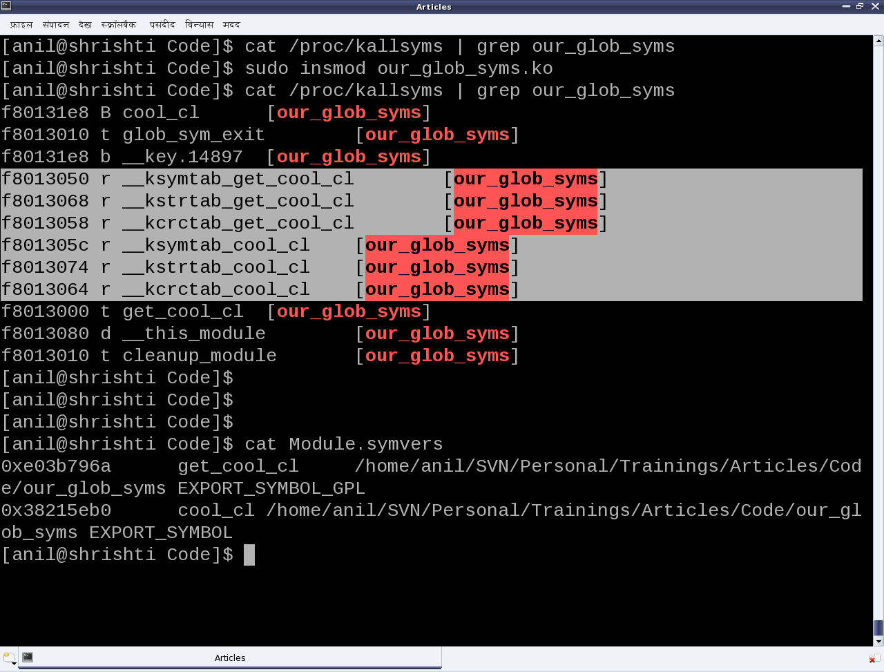
Each exported symbol also have a corresponding structure placed into each of the kernel symbol table (__ksymtab), kernel string table (__kstrtab), and kernel CRC table (__kcrctab) sections, marking it to be globally accessible. Figure 30 shows a filtered snippet of the /proc/kallsyms kernel window, before and after loading the module our_glob_syms.ko, which has been compiled using the driver’s usual makefile.

Figure 30: Our global symbols module

Figure 30: Our global symbols module

The following code shows the supporting header file (our_glob_syms.h), to be included by modules using the exported symbols cool_cl and get_cool_cl:

#ifndef OUR_GLOB_SYMS_H
#define OUR_GLOB_SYMS_H

#ifdef __KERNEL__
#include <linux/device.h>

extern struct class *cool_cl;
extern struct class *get_cool_cl(void);
#endif

#endif

Figure 30 also shows the file Module.symvers, generated by compilation of the module our_glob_syms. This contains the various details of all the exported symbols in its directory. Apart from including the above header file, the modules using the exported symbols, possibly should have this file Module.symvers in their build directory.

Note the <linux/device.h> header in the above examples, is being included for the various class related declarations & definitions, which has been already covered under the character drivers discussions.

Module Parameters

Being aware of passing command line arguments to an application, it is a natural quest to ask if something similar can be done with a module. And the answer is yes. Parameters can be passed to a module along with loading it, say using insmod. Interestingly enough and in contrast with the command line arguments to an application, these can be modified even later as well, through sysfs interactions.

The module parameters are setup using the following macro (defined in <linux/moduleparam.h>, included through <linux/module.h>):

module_param(name, type, perm)

where, name is the parameter name, type is the type of the parameter, and perm is the permissions of the sysfs file corresponding to this parameter. Supported type values are: byte, short, ushort, int, uint, long, ulong, charp (character pointer), bool or invbool (inverted boolean). The following module code (module_param.c) demonstrates a module parameter:

#include <linux/module.h>
#include <linux/kernel.h>

static int cfg_value = 3;
module_param(cfg_value, int, 0764);

static int __init mod_par_init(void)
{
	printk(KERN_INFO "Loaded with %d\n", cfg_value);
	return 0;
}

static void __exit mod_par_exit(void)
{
	printk(KERN_INFO "Unloaded cfg value: %d\n", cfg_value);
}

module_init(mod_par_init);
module_exit(mod_par_exit);

MODULE_LICENSE("GPL");
MODULE_AUTHOR("Anil Kumar Pugalia <email@sarika-pugs.com>");
MODULE_DESCRIPTION("Module Parameter demonstration Driver");

Note that before the parameter setup, a variable of the same name and compatible type needs to be defined.

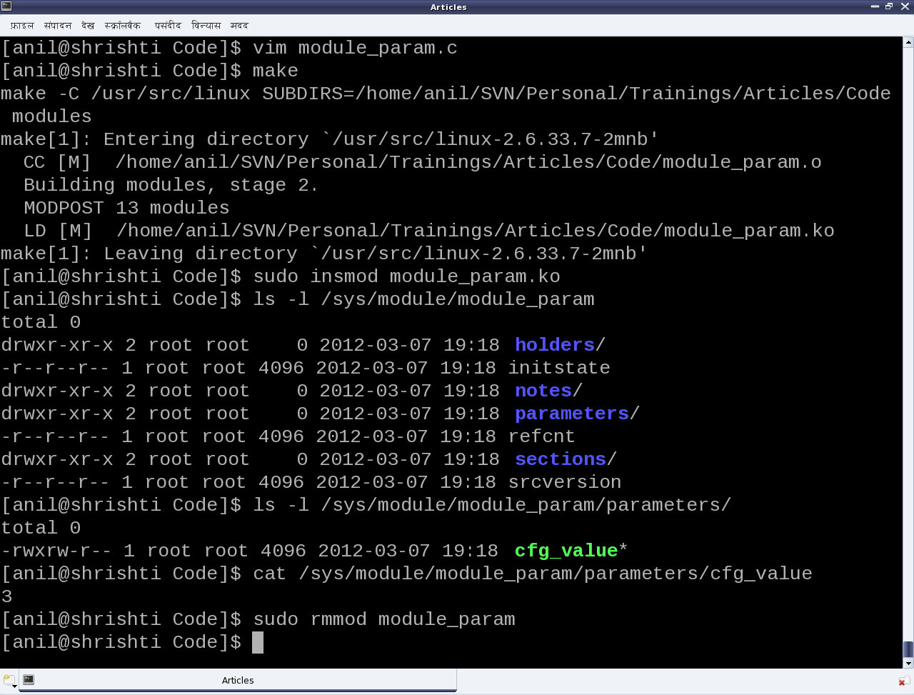
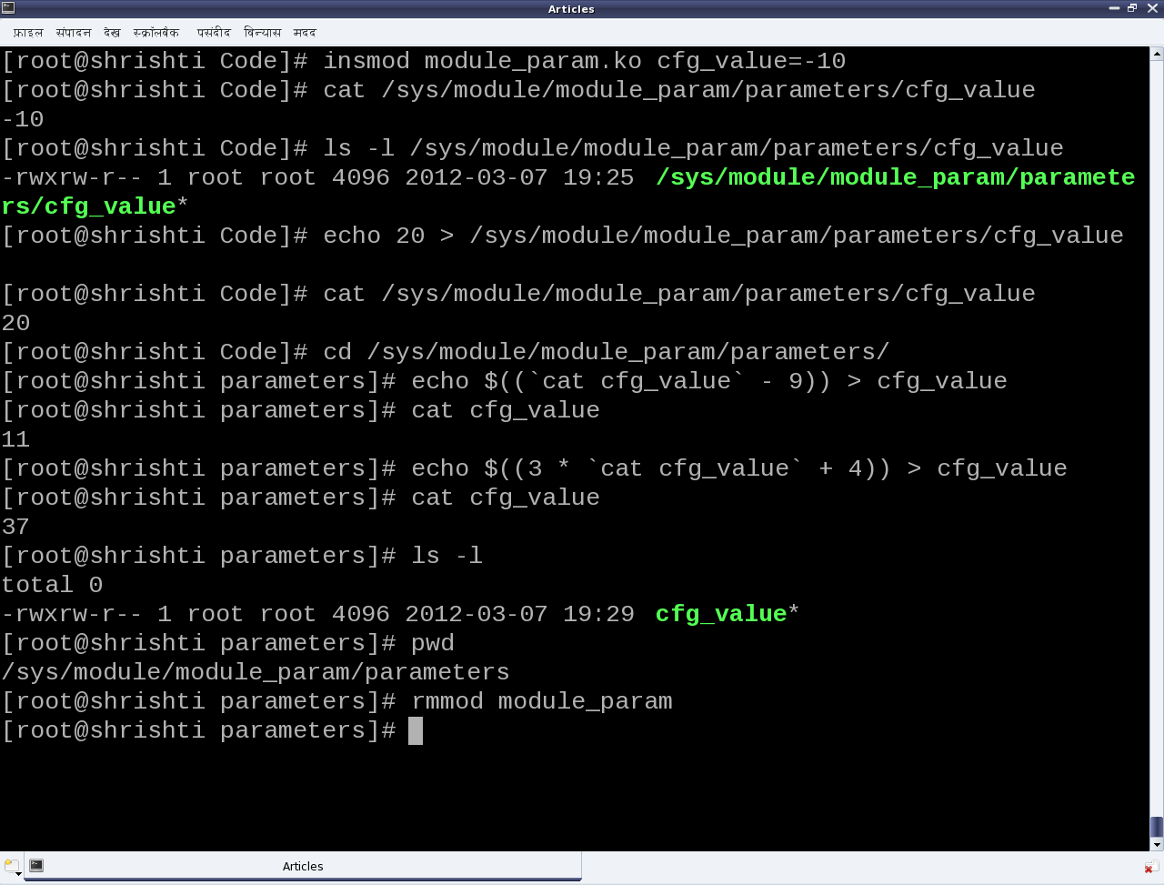
Subsequently, the following steps and experiments are shown in Figures 31 and 32:

  • Building the driver (module_param.ko file) using the driver’s usual makefile
  • Loading the driver using insmod (with and without parameters)
  • Various experiments through the corresponding /sys entries
  • And finally, unloading the driver using rmmod
Figure 31: Experiments with module parameter

Figure 31: Experiments with module parameter

Figure 32: Experiments with module parameter (as root)

Figure 32: Experiments with module parameter (as root)

Observe the following:

  • Initial value (3) of cfg_value becomes its default value when insmod is done without any parameters
  • Permission 0764 gives rwx to the user, rw- to the group, and r– for the others on the file cfg_value under parameters of module_param under /sys/module/

Check for yourself:

  • Output of dmesg | tail on every insmod and rmmod for the output of printk‘s
  • Try writing into the /sys/module/module_param/parameters/cfg_value file as a normal user

Summing up

With this, the duo have a fairly good understanding of Linux drivers and they are all set to start working on their final semester project. Any guesses on what their topic is all about? Hint: They have picked up one of the most daunting Linux driver topic. Let us see, how they fair at it.

Eighteenth Article >>

   Send article as PDF   

High School Trigo with Maxima

This seventeenth article of the mathematical journey through open source, takes through a tour of the high school trigonometry using Maxima.

<< Sixteenth Article

Trigonometry first gets introduced to students of standard IX, through triangles. And, then it takes its own journey through the jungle of formulae and tables. And one knows, being good at instant recall of various formulae, makes her good at trigo. The idea here is not to be good at mugging up the formulae but rather applying them to get the various end results. It assumes that you possibly already know the formulae.

Fundamental trigonometric functions

Maxima provides all the familiar fundamental trigonometric functions, including the hyperbolic ones. They can be tabulated as follows:

Mathematical Names

Normal

Hyperbolic

Functions

Inv. Functions

Functions

Inv. Functions

sine (sin)

sin()

asin()

sinh()

asinh()

cosine (cos)

cos()

acos()

cosh()

acosh()

tangent (tan)

tan()

atan()

tanh()

atanh()

cosecant (cosec)

csc()

acsc()

csch()

acsch()

secant (sec)

sec()

asec()

sech()

asech()

cotangent (cot)

cot()

acot()

coth()

acoth()

Note that all of their arguments are values in radians. And here follows a demonstration of a small subset of those:

$ maxima -q
(%i1) cos(0);
(%o1)                                  1
(%i2) cos(%pi/2);
(%o2)                                  0
(%i3) cot(0);
The number 0 isn't in the domain of cot
 -- an error. To debug this try: debugmode(true);
(%i4) tan(%pi/4);
(%o4)                                  1
(%i5) string(asin(1));
(%o5)                                %pi/2
(%i6) csch(0);
The number 0 isn't in the domain of csch
 -- an error. To debug this try: debugmode(true);
(%i7) csch(1);
(%o7)                               csch(1)
(%i8) asinh(0);
(%o8)                                  0
(%i9) string(%i * sin(%pi / 3)^2 + cos(5 * %pi / 6));
(%o9)                         3*%i/4-sqrt(3)/2
(%i10) quit();

Simplifications with special angles like %pi / 10 and its multiples could be enabled by loading the ntrig package. Check out the difference below, before and after loading the package:

$ maxima -q
(%i1) string(sin(%pi/10));
(%o1)                             sin(%pi/10)
(%i2) string(cos(2*%pi/10));
(%o2)                             cos(%pi/5)
(%i3) string(tan(3*%pi/10));
(%o3)                            tan(3*%pi/10)
(%i4) load(ntrig);
(%o4)        /usr/share/maxima/5.24.0/share/trigonometry/ntrig.mac
(%i5) string(sin(%pi/10));
(%o5)                            (sqrt(5)-1)/4
(%i6) string(cos(2*%pi/10));
(%o6)                            (sqrt(5)+1)/4
(%i7) string(tan(3*%pi/10));
(%o7)          sqrt(2)*(sqrt(5)+1)/((sqrt(5)-1)*sqrt(sqrt(5)+5))
(%i8) quit();

A very common trigonometric problem is, given a tangent value find the corresponding angle. Now, a common challenge is for every value, the angle could lie in two quadrants. For a positive tangent, the angle could be in the first or the third quadrant, and for a negative value, the angle could be in the second or the fourth quadrant. So, atan() cannot always calculate the correct quadrant of the angle. Now, how do we know it exactly. Obviously, we need some extra information, say the actual values of the perpendicular (p) and the base (b) of the tangent, rather than just the tangent value. With that, the angle location could be tabulated as follows:

Perpendicular (p)

Base (b)

Tangent (p/b)

Angle Quadrant

Positive

Positive

Positive

First

Positive

Negative

Negative

Second

Negative

Negative

Positive

Third

Negative

Positive

Negative

Fourth

And this functionality is captured in the atan2() function, which takes 2 arguments, the p and the b, and thus does provide the angle in the correct quadrant, as per the table above. Along with this, the infinities of tangent are also taken care. Here’s a demo:

$ maxima -q
(%i1) atan2(0, 1); /* Zero */
(%o1)                                  0
(%i2) atan2(0, -1); /* Zero */
(%o2)                                 %pi
(%i3) string(atan2(1, -1)); /* -1 */
(%o3)                               3*%pi/4
(%i4) string(atan2(-1, -1)); /* 1 */
(%o4)                              -3*%pi/4
(%i5) string(atan2(-1, 0)); /* - Infinity */
(%o5)                               -%pi/2
(%i6) string(atan2(5, 0)); /* + Infinity */
(%o6)                                %pi/2
(%i7) quit();

Trigonometric Identities

Maxima supports many built-in trigonometric identities, and one can add his own as well. First one to look at would be the set dealing with integral multiples and factors of %pi. We’ll declare a few integers and then play around with them.

$ maxima -q
(%i1) declare(m, integer, n, integer);
(%o1)                                done
(%i2) properties(m);
(%o2)                  [database info, kind(m, integer)]
(%i3) sin(m * %pi);
(%o3)                                  0
(%i4) string(cos(n * %pi));
(%o4)                              (-1)^n
(%i5) string(cos(m * %pi / 2)); /* No simplification */
(%o5)                            cos(%pi*m/2)
(%i6) declare(m, even); /* Will lead to simplification */
(%o6)                               done
(%i7) declare(n, odd);
(%o7)                               done
(%i8) cos(m * %pi);
(%o8)                                 1
(%i9) cos(n * %pi);
(%o9)                                - 1
(%i10) string(cos(m * %pi / 2));
(%o10)                             (-1)^(m/2)
(%i11) string(cos(n * %pi / 2));
(%o11)                            cos(%pi*n/2)
(%i12) quit();

Next is the relation between the normal & the hyperbolic trigo functions.

$ maxima -q
(%i1) sin(%i * x);
(%o1)                            %i sinh(x)
(%i2) cos(%i * x);
(%o2)                              cosh(x)
(%i3) tan(%i * x);
(%o3)                            %i tanh(x)
(%i4) quit();

By enabling the option variable halfangles, many half angle identities, come into play. To be specific, sin(x/2) gets further simplified in (0, 2 * %pi) range, cos(x/2) gets further simplified in (-%pi/2, %pi/2) range. Check out the differences, before and after enabling the option variable, along with the range modifications, in the examples below:

$ maxima -q
(%i1) string(2*cos(x/2)^2 - 1); /* No effect */
(%o1)                           2*cos(x/2)^2-1
(%i2) string(cos(x/2)); /* No effect */
(%o2)                              cos(x/2)
(%i3) halfangles:true; /* Enabling half angles */
(%o3)                                true
(%i4) string(2*cos(x/2)^2 - 1); /* Simplified */
(%o4)                               cos(x)
(%i5) string(cos(x/2)); /* Complex expansion for all x */
(%o5)         (-1)^floor((x+%pi)/(2*%pi))*sqrt(cos(x)+1)/sqrt(2)
(%i6) assume(-%pi < x, x < %pi); /* Limiting x values */
(%o6)                        [x > - %pi, x < %pi]
(%i7) string(cos(x/2)); /* Further simplified */
(%o7)                       sqrt(cos(x)+1)/sqrt(2)
(%i8) quit();

Trigonometric Expansions and Simplifications

Trigonometry is full of multiples of angles, sums of angles, products & powers of trigo functions, and the long list of relations between them. Multiples and sums of angles fall into one category. Products and powers of trigo functions in an another category. And its very useful to do conversions from one of these categories to the other one, to crack a range of simple to complex problems, catering to basic hobby science to quantum mechanics. trigexpand() does the conversion from “multiples & sums of angles” to “products & powers of trigo functions”. trigreduce() does exactly the opposite. Here’s goes a small demo:

$ maxima -q
(%i1) trigexpand(sin(2*x));
(%o1)                           2 cos(x) sin(x)
(%i2) trigexpand(sin(x+y)-sin(x-y));
(%o2)                           2 cos(x) sin(y)
(%i3) trigexpand(cos(2*x+y)-cos(2*x-y));
(%o3)                         - 2 sin(2 x) sin(y)
(%i4) trigexpand(%o3);
(%o4)                      - 4 cos(x) sin(x) sin(y)
(%i5) string(trigreduce(%o4));
(%o5)                  -2*(cos(y-2*x)/2-cos(y+2*x)/2)
(%i6) string(trigsimp(%o5));
(%o6)                       cos(y+2*x)-cos(y-2*x)
(%i7) string(trigexpand(cos(2*x)));
(%o7)                         cos(x)^2-sin(x)^2
(%i8) string(trigexpand(cos(2*x) + 2*sin(x)^2));
(%o8)                         sin(x)^2+cos(x)^2
(%i9) trigsimp(trigexpand(cos(2*x) + 2*sin(x)^2));
(%o9)                                 1
(%i10) quit();

In %o5 above, you might have noted that the 2’s could have been cancelled for further simplification. But that is not the job of trigreduce(), and for that we have to apply the trigsimp() function as shown in %i6. In fact, many other trigonometric identities based simplification are achieved using trigsimp(). Check out the %i7 to %o9 sequences for another such example.

Eighteenth Article >>

   Send article as PDF   

Kernel Window: Peeping through /proc

This sixteenth article, which is part of the series on Linux device drivers, demonstrates the creation and usage of files under the /proc virtual file-system.

<< Fifteenth Article

Useful kernel windows

After many months, Shweta and Pugs got together for a peaceful technical romancing. All through, we have been using all kinds of kernel windows especially through the /proc virtual file-system (using cat), to help us out in decoding the various nitty-gritties of Linux device drivers. Here’s a non-exhaustive summary listing:

  • /proc/modules – Listing of all the dynamically loaded modules
  • /proc/devices – Listing of all the registered character and block major numbers
  • /proc/iomem – Listing of on-system physical RAM & bus device addresses
  • /proc/ioports – Listing of on-system I/O port addresses (specially for x86 systems)
  • /proc/interrupts – Listing of all the registered interrupt request numbers
  • /proc/softirqs – Listing of all the registered soft irqs
  • /proc/kallsyms – Listing of all the running kernel symbols, including from loaded modules
  • /proc/partitions – Listing of currently connected block devices & their partitions
  • /proc/filesystems – Listing of currently active file-system drivers
  • /proc/swaps – Listing of currently active swaps
  • /proc/cpuinfo – Information about the CPU(s) on the system
  • /proc/meminfo – Information about the memory on the system, viz. RAM, swap, …

Custom kernel windows

“Yes, these have been really helpful in understanding and debugging the Linux device drivers. But is it possible for us to also provide some help? Yes, I mean can we create one such kernel window through /proc?”, questioned Shweta.

“Why one? As many as you want. And that’s simple – just use the right set of APIs and there you go.”

“For you every thing is simple.”

“No yaar, this is seriously simple”, smiled Pugs. “Just watch out, me creating one for you.”

And in jiffies, Pugs created the proc_window.c file below (including the changes, which has taken place in kernel v3.10 and v4.3):

#include <linux/module.h>
#include <linux/kernel.h>
#include <linux/version.h>
#if (LINUX_VERSION_CODE < KERNEL_VERSION(3,10,0))
#else
#include <linux/fs.h>
#include <linux/seq_file.h>
#endif
#include <linux/proc_fs.h>
#include <linux/jiffies.h>
#include <linux/uaccess.h>

#if (LINUX_VERSION_CODE < KERNEL_VERSION(3,10,0))
#define STR_PRINTF_RET(len, str, args...) len += sprintf(page + len, str, ## args)
#elif (LINUX_VERSION_CODE < KERNEL_VERSION(4,3,0))
#define STR_PRINTF_RET(len, str, args...) len += seq_printf(m, str, ## args)
#else
#define STR_PRINTF_RET(len, str, args...) seq_printf(m, str, ## args)
#endif

static struct proc_dir_entry *parent, *file, *link;
static int state = 0;

#if (LINUX_VERSION_CODE < KERNEL_VERSION(3,10,0))
static int time_read(char *page, char **start, off_t off, int count, int *eof,
	void *data)
#else
static int time_read(struct seq_file *m, void *v)
#endif
{
	int len = 0, val;
	unsigned long act_jiffies;

	STR_PRINTF_RET(len, "state = %d\n", state);
	act_jiffies = jiffies - INITIAL_JIFFIES;
	val = jiffies_to_msecs(act_jiffies);
	switch (state)
	{
		case 0:
			STR_PRINTF_RET(len, "time = %ld jiffies\n", act_jiffies);
			break;
		case 1:
			STR_PRINTF_RET(len, "time = %d msecs\n", val);
			break;
		case 2:
			STR_PRINTF_RET(len, "time = %ds %dms\n",
					val / 1000, val % 1000);
			break;
		case 3:
			val /= 1000;
			STR_PRINTF_RET(len, "time = %02d:%02d:%02d\n",
					val / 3600, (val / 60) % 60, val % 60);
			break;
		default:
			STR_PRINTF_RET(len, "\n");
			break;
	}

	return len;
}
#if (LINUX_VERSION_CODE < KERNEL_VERSION(3,10,0))
static int time_write(struct file *file, const char __user *buffer,
	unsigned long count, void *data)
#else
static ssize_t time_write(struct file *file, const char __user *buffer,
	size_t count, loff_t *off)
#endif
{
	char kbuf[2];

	if (count > 2)
		return count;
	if (copy_from_user(kbuf, buffer, count))
	{
		return -EFAULT;
	}
	if ((count == 2) && (kbuf[1] != '\n'))
		return count;
	if ((kbuf[0] < '0') || ('9' < kbuf[0]))
		return count;
	state = kbuf[0] - '0';
	return count;
}
#if (LINUX_VERSION_CODE < KERNEL_VERSION(3,10,0))
#else
static int time_open(struct inode *inode, struct file *file)
{
	return single_open(file, time_read, NULL);
}

static struct file_operations fops =
{
	.owner = THIS_MODULE,
	.open = time_open,
	.read = seq_read,
	.write = time_write
};
#endif

static int __init proc_win_init(void)
{
	if ((parent = proc_mkdir("anil", NULL)) == NULL)
	{
		return -1;
	}
#if (LINUX_VERSION_CODE < KERNEL_VERSION(3,10,0))
	if ((file = create_proc_entry("rel_time", 0666, parent)) == NULL)
#else
	if ((file = proc_create("rel_time", 0666, parent, &fops)) == NULL)
#endif
	{
		remove_proc_entry("anil", NULL);
		return -1;
	}
#if (LINUX_VERSION_CODE < KERNEL_VERSION(3,10,0))
	file->read_proc = time_read;
	file->write_proc = time_write;
#endif
	if ((link = proc_symlink("rel_time_l", parent, "rel_time")) == NULL)
	{
		remove_proc_entry("rel_time", parent);
		remove_proc_entry("anil", NULL);
		return -1;
	}
#if (LINUX_VERSION_CODE < KERNEL_VERSION(3,10,0))
	link->uid = 0;
	link->gid = 100;
#else
	proc_set_user(link, KUIDT_INIT(0), KGIDT_INIT(100));
#endif
	return 0;
}

static void __exit proc_win_exit(void)
{
	remove_proc_entry("rel_time_l", parent);
	remove_proc_entry("rel_time", parent);
	remove_proc_entry("anil", NULL);
}

module_init(proc_win_init);
module_exit(proc_win_exit);

MODULE_LICENSE("GPL");
MODULE_AUTHOR("Anil Kumar Pugalia <email@sarika-pugs.com>");
MODULE_DESCRIPTION("Kernel window /proc Demonstration Driver");

And then Pugs did the following steps:

  • Built the driver (proc_window.ko file) using the usual driver’s Makefile.
  • Loaded the driver using insmod.
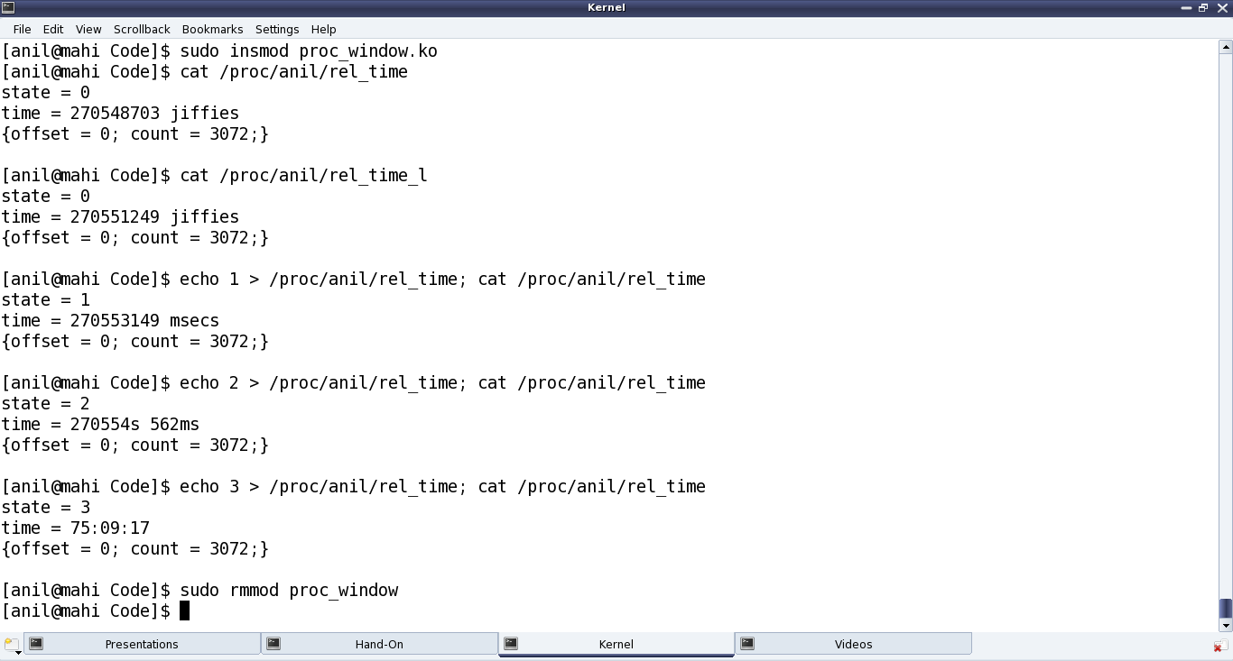
  • Showed various experiments using the newly created proc windows. (Refer to Figure 28.)
  • And finally, unloaded the driver using rmmod.
Figure 28: Peeping through /proc

Figure 28: Peeping through /proc

Demystifying the details

Starting from the constructor proc_win_init(), three proc entries are created:

  • Directory anil under /proc (i.e. NULL parent) with default permissions 0755, using proc_mkdir()
  • Regular file rel_time under the above directory anil with permissions 0666, using create_proc_entry() or proc_create() (since kernel v3.10)
  • Soft link rel_time_l to the above file rel_time under the same directory anil, using proc_symlink()

The corresponding removal of these three is achieved using remove_proc_entry() in the destructor proc_win_exit(), in chronological reverse order.

For every entry created under /proc, a corresponding struct proc_dir_entry is created. After which many of its fields could be further updated as needed:

  • mode – Permissions of the file
  • uid – User ID of the file
  • gid – Group ID of the file

Since kernel v3.10, specific API proc_set_user() has been provided to update the uid & gid, instead of directly modifying the fields.

Additionally, for a regular file, the following two function pointers for read and write over the file could be provided, respectively:

  • int (*read_proc)(char *page, char **start, off_t off, int count, int *eof, void *data)
  • int (*write_proc)(struct file *file, const char __user *buffer, unsigned long count, void *data)

Again, since kernel v3.10, the read & write fields of struct file_operations are to be used respectively, instead of the above two.

write_proc() is very similar to the character device file operation write. And the above code implementation, lets the user to write a digit from 0 to 9, and accordingly sets the internal state.

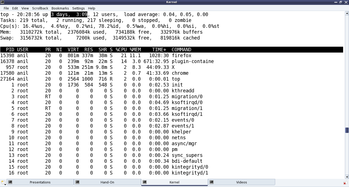
read_proc() in the above code implementation provides the current state and the time since the system has been booted up in different units based on the current state. These are, jiffies in state 0; milliseconds in state 1; seconds & milliseconds in state 2; hours : minutes : seconds in state 3; and <not implemented> in other states. And to check the computation accuracy, Figure 29 highlights the system up time in the output of top. read_proc()‘s page parameter is a page-sized buffer, typically to be filled up with count bytes from offset off. But more often than not (because of small content), just page is filled up, ignoring all other parameters. Since kernel v3.10, the read logic has to be implemented through something called a sequence file, which is implemented by specifying the pre-defined seq_read() function for the file operation read, and then by providing the above logic in the sequence file’s read function through the file operation open using single_open().

Figure 29: Comparison with top's output

Figure 29: Comparison with top’s output

All the /proc related structure definitions and function declarations are available through <linux/proc_fs.h>. The sequence file related stuff (since kernel v3.10) are available through <linux/seq_file.h>. And the jiffies related function declarations and macro definitions are in <linux/jiffies.h>. On a special note, the actual jiffies are being calculated by subtracting INITIAL_JIFFIES, as on boot-up, jiffies is initialized to INITIAL_JIFFIES instead of zero.

Summing up

“Hey Pugs!!! Why did you create the folder named as anil? Who is this Anil? You could have used my name or may be yours.” suggested Shweta. “Ha!! That’s a surprise. My real name is Anil only. It is just that everyone in college knows me only as Pugs”, smiled Pugs. Watch out for further technical romancing of Pugs aka Anil.

Seventeenth Article >>

Notes

  1. One of the powerful usage of creating our own proc window is for customized debugging by querying. A simple but cool modification of the above driver, could be instead of getting the jiffies, it could read / write hardware registers.
   Send article as PDF   

Polynomials in Maxima

This sixteenth article of the mathematical journey through open source, demonstrates the polynomial manipulations using Maxima.

<< Fifteenth Article

Polynomials have fascinated mathematicians since ages. Moreover, because of wide variety of their applications, ranging from basic algebra to puzzles to various sciences. Here, we are going to look at some of the polynomial manipulation functions provided by Maxima, and a couple of real world applications using some of them.

Fundamental polynomial operations

Let’s start with a demonstration of the fundamental polynomial operations, like addition, subtraction, multiplication, division. In all these, whenever needed,we’ll use expand() to expand the polynomials, and string() to display the polynomials in a flattened notation.

$ maxima -q
(%i1) p1: x^2 - y^2 + y$
(%i2) p2: -x^2 - y^2 + x$
(%i3) p3: (x + y)^2$
(%i4) string(p1 + p2);
(%o4)                             -2*y^2+y+x
(%i5) string(p1 + p2 + p3);
(%o5)                          (y+x)^2-2*y^2+y+x
(%i6) string(expand(p1 + p2 + p3));
(%o6)                         -y^2+2*x*y+y+x^2+x
(%i7) string(expand(p3 - p1));
(%o7)                            2*y^2+2*x*y-y
(%i8) string(expand(p1 * p2));
(%o8)                   y^4-y^3-x*y^2-x^2*y+x*y-x^4+x^3
(%i9) string(p1 / p2);
(%o9)                     (-y^2+y+x^2)/(-y^2-x^2+x)
(%i10) string(divide(p1, p2));
(%o10)                           [1,y+2*x^2-x]
(%i11) string(divide(x^2 - y^2, x + y));
(%o11)                              [x-y,0]
(%i12) quit();

Note that the / operator just places the polynomials as a fraction, rather then dividing them. And the function divide() actually divides the first polynomial by the second one, yielding a list with the quotient and the remainder of the division. If the division needs to be with respect to a particular variable, that can be passed as the third argument to divide. Check out the variation below, to understand what it means:

$ maxima -q
(%i1) string(divide(x^2 - y^2 + y, x + y, x));
(%o1)                              [x-y,y]
(%i2) string(divide(x^2 - y^2 + y, x + y, y));
(%o2)                            [-y+x+1,-x]
(%i3) quit();

Coefficients of a polynomial

Extracting the coefficients of a polynomial is another basic and common requirement for polynomial manipulations. Maxima provides two slightly different mechanisms. First one, just finds the coefficient of a given variable or its some power, using coeff(). Second one, segregates a polynomial into the coefficient of a given variable or its power, and the remaining terms, using bothcoef().

$ maxima -q
(%i1) string(bothcoef(expand(x^2 - y^2 + (x + y)^2), x^2));
(%o1)                             [2,2*x*y]
(%i2) string(bothcoef(expand(x^2 - y^2 + (x + y)^2), x));
(%o2)                            [2*y,2*x^2]
(%i3) string(bothcoef(expand(x^2 - y^2 + (x + y)^2), y^2));
(%o3)                          [0,2*x*y+2*x^2]
(%i4) string(bothcoef(expand(x^2 - y^2 + (x + y)^2), y));
(%o4)                            [2*x,2*x^2]
(%i5) string(coeff(expand((x + 2 * y)^50), x^20));
(%o5)                   50604606318512743383040*y^30
(%i6) string(coeff(expand((a + b + c + d)^4), a^3));
(%o6)                            4*d+4*c+4*b
(%i7) quit();

Polynomial fractions

Calculating the greatest common divisor (GCD) is one of the very useful operations to simply fractions of polynomials. Other common requirements are extracting the numerator, the denominator, and the highest power. Here goes the function demonstrations for all of these:

$ maxima -q
(%i1) gcd(x^3 + 3*x^2 + 3*x + 1, x^2 + 3*x + 2);
(%o1)                              x + 1
(%i2) string(ezgcd(x^3 + 3*x^2 + 3*x + 1, x^2 + 3*x + 2));
(%o2)                       [x+1,x^2+2*x+1,x+2]
(%i3) string(denom((x + 1)^-3 * (1 - x)^2));
(%o3)                             (x+1)^3
(%i4) string(num((x + 1)^-3 * (1 - x)^2));
(%o4)                             (1-x)^2
(%i5) hipow(expand((x + 1)^3 + (1 - x)^3), x);
(%o5)                                2
(%i6) quit();

Note that the ezgcd() function lists out the remainder polynomials, along with the GCD.

Polynomial fractions could be differentiated using the powerful ratdiff().

$ maxima -q
(%i1) string(ratdiff((x + 1)^-1 * (1 - x)^2, x));
(%o1)                     (x^2+2*x-3)/(x^2+2*x+1)
(%i2) string(ratdiff(1 / (x + 1), x));
(%o2)                         -1/(x^2+2*x+1)
(%i3) string(ratdiff((x^2 - 1) / (x + 1), x));
(%o3)                                1
(%i4) quit();

And, ratsubst() is a powerful expression substitution function, with intelligence. It would dig into the expression to simplify complicated expressions, including trigonometric ones. Check out the %i5, for one of its powerful application. ratsubst(<new>, <old>, <expr>) replaces the <old> expression by the <new> expression in the complete expression <expr>.

$ maxima -q
(%i1) string(ratsubst(u, x^2, x^3 + 3*x^2 + 3*x + 1));
(%o1)                          (u+3)*x+3*u+1
(%i2) string(ratsubst(u, x^2, (x+1)^3));
(%o2)                          (u+3)*x+3*u+1
(%i3) string(ratsubst(u, x^2, (x+1)^4));
(%o3)                       (4*u+4)*x+u^2+6*u+1
(%i4) string(ratsubst(u, x - 1, x^4 - 2*x^2 + 1));
(%o4)                         u^4+4*u^3+4*u^2
(%i5) string(ratsubst(sin(x)^2, 1 - cos(x)^2, cos(x)^4 - 2*cos(x)^2 + 1));
(%o5)                            sin(x)^4
(%i5) quit();

Variable eliminations & equation solving

Very often, we come across N sets of equations in M sets of unknowns, where M >= N. If M = N, then most likely there exists a unique solution. However, if M > N, then there may be many possible solutions, but with some constraints. And in such case, it would be helpful to deduce some simpler set of expressions. This can be achieved using eliminate() of Maxima. Let’s have two polynomial expressions in 3 variables x, y, z to demonstrate the same.

$ maxima -q
(%i1) p1: x^2 + 2*x*y + z^2$
(%i2) p2: x + y + z$
(%i3) string(eliminate([p1, p2], [x]));
(%o3)                            [2*z^2-y^2]
(%i4) string(eliminate([p1, p2], [y]));
(%o4)                         [-z^2+2*x*z+x^2]
(%i5) string(eliminate([p1, p2], [z]));
(%o5)                         [y^2+4*x*y+2*x^2]
(%i6) quit();

Note that in all the above polynomial expressions, the expressions are assumed to be equated to zero. A beautiful application of the above is solving recurrence relations. Let’s say we have a non-linear equation given by Yn+1 = r * Yn * (1 – Yn). And, we want to solve it for a scenario that as n tends to infinity, the value of Y oscillates between two distinct values. This means that Yn+2 = Yn. Hence, we would have two expressions with three unknowns to solve with, namely:

  1. Yn+1 = r * Yn * (1 – Yn)
  2. Yn = r * Yn+1 * (1 – Yn+1)

So, representing Yn+1 with yn1 and Yn by yn, we may use solve() to solve for yn & yn1 in terms of r. But, if rather we want to get a feel of the equation which pops up, in terms of yn, we would have to use eliminate() to eliminate yn1.

$ maxima -q
(%i1) p1: yn1 = r * yn * (1 - yn)$
(%i2) p2: yn = r * yn1 * (1 - yn1)$
(%i3) string(eliminate([p1, p2], [yn1]));
(%o3)          [yn*(r^3*yn^3-2*r^3*yn^2+(r^3+r^2)*yn-r^2+1)]
(%i4) string(solve([p1, p2], [yn, yn1])); /* Just to show the solution */
(%o4) [[yn = (r-1)/r,yn1 = (r-1)/r],
    [yn = -(sqrt(r^2-2*r-3)-r-1)/(2*r),yn1 = (sqrt(r-3)*sqrt(r+1)+r+1)/(2*r)],
    [yn = (sqrt(r^2-2*r-3)+r+1)/(2*r),yn1 = -(sqrt(r-3)*sqrt(r+1)-r-1)/(2*r)],
    [yn = 0,yn1 = 0]]
(%i5) quit()

Seventeenth Article >>

   Send article as PDF   

Disk on RAM: Playing destructively

This fifteenth article, which is part of the series on Linux device drivers, experiments with a dummy hard disk on RAM to demonstrate the block drivers.

<< Fourteenth Article

Play first, rules later

After a delicious lunch, theory makes audience sleepy. So, let’s start with the code itself. Code demonstrated is available at dor_code.tar.bz2. This tar ball contains 3 ‘C’ source files, 2 ‘C’ headers, and a Makefile. As usual, executing make will build the ‘disk on ram’ driver (dor.ko) – this time combining the 3 ‘C’ files. Check out the Makefile to see how. make clean would do the usual clean of the built stuff.

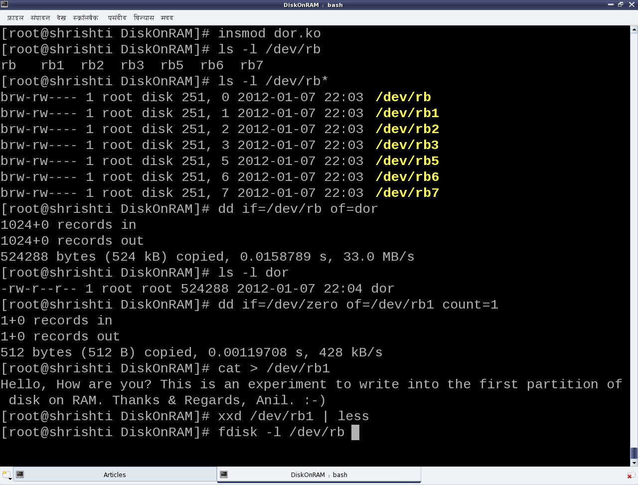
Once built, the following are the experimenting steps (Refer to Figures 25, 26, 27):

  • Load the driver dor.ko using insmod. This would create the block device files representing the disk on 512 KibiBytes (KiB) of RAM, with 3 primary and 3 logical partitions.
  • Checkout the automatically created block device files (/dev/rb*). /dev/rb is the entire disk of 512 KiB size. rb1, rb2, rb3 are the primary partitions with rb2 being the extended partition and containing the 3 logical partitions rb5, rb6, rb7.
  • Read the entire disk (/dev/rb) using the disk dump utility dd.
  • Zero out the first sector of the disk’s first partition (/dev/rb1) again using dd.
  • Write some text into the disk’s first partition (/dev/rb1) using cat.
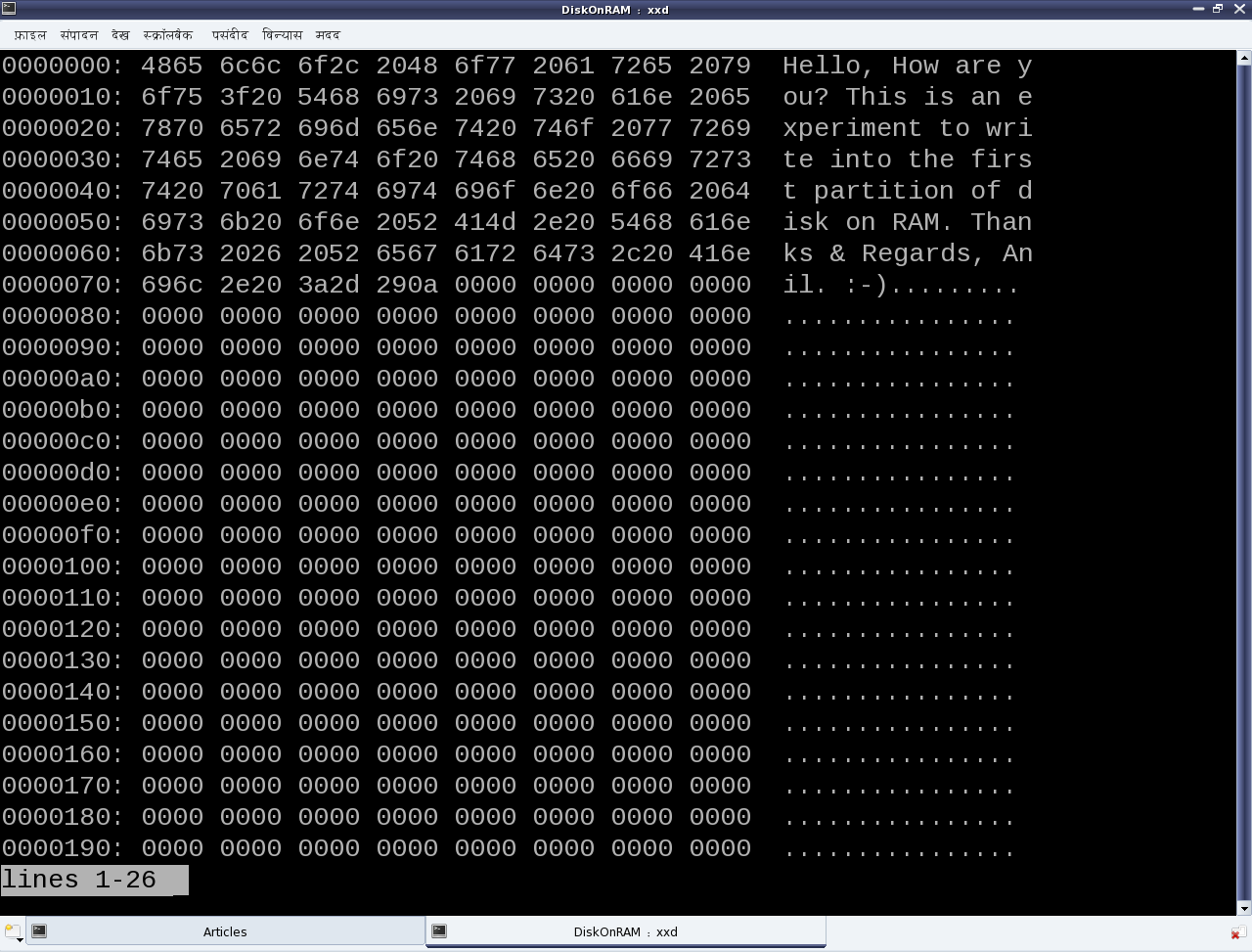
  • Display the initial contents of the first partition (/dev/rb1) using the xxd utility. See Figure 26 for the xxd output.
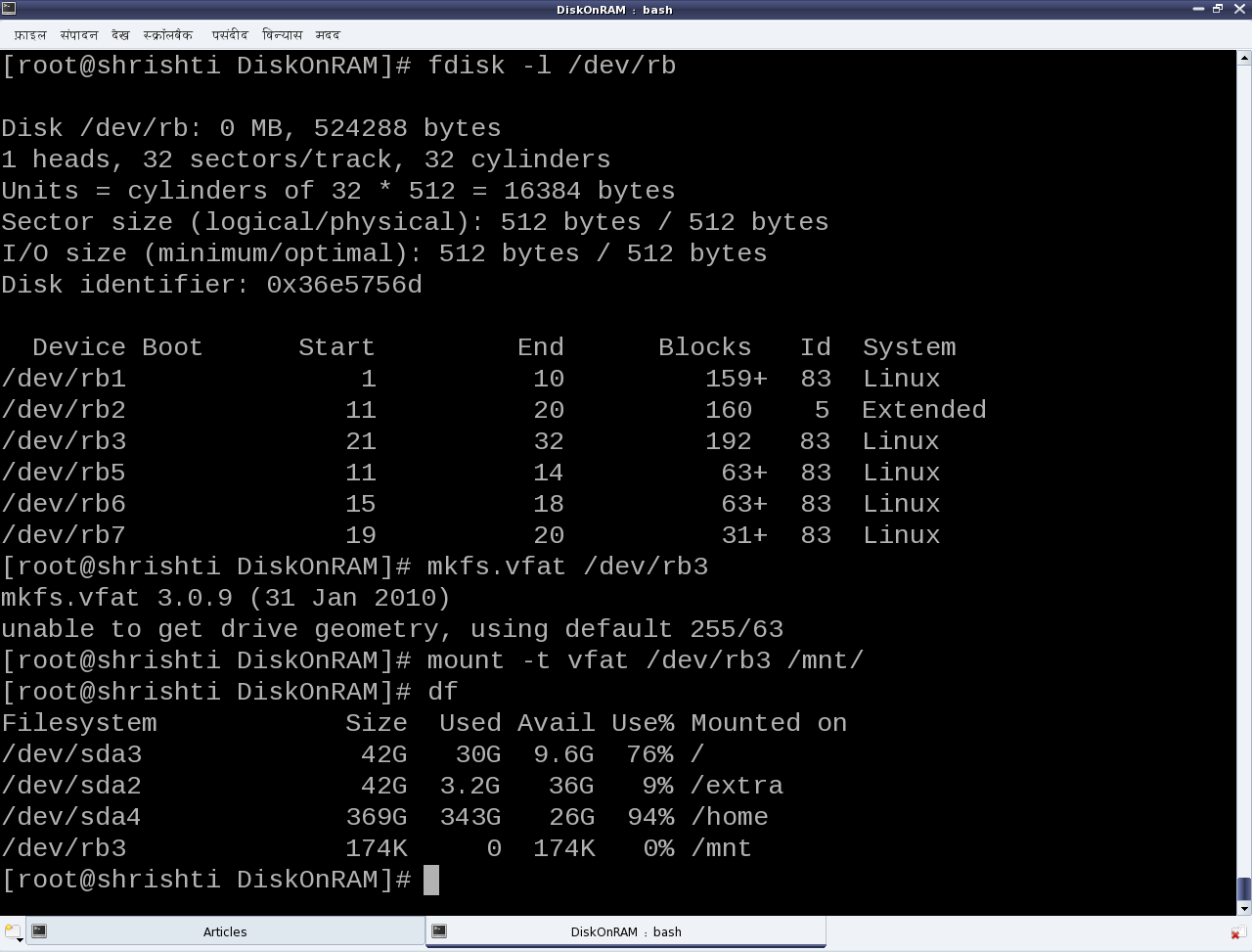
  • Display the partition info for the disk using fdisk. See Figure 27 for the fdisk output.
  • (Quick) Format the third primary partition (/dev/rb3) as vfat filesystem (like your pen drive), using mkfs.vfat (Figure 27).
  • Mount the newly formatted partition using mount, say at /mnt (Figure 27).
  • Disk usage utility df would now show this partition mounted at /mnt (Figure 27). You may go ahead and store your files there. But, please remember that these partitions are all on a disk on RAM, and so non-persistent. Hence,
  • Unloading the driver using ‘rmmod dor‘ would vanish everything. Though the partition needs to be unmounted using ‘umount /mnt‘ before doing that.

Please note that all the above experimenting steps need to be executed with root privileges.

Figure 25: Playing with 'Disk on RAM' driver

Figure 25: Playing with ‘Disk on RAM’ driver

Figure 26: xxd showing the initial data on the first partition (/dev/rb1)

Figure 26: xxd showing the initial data on the first partition (/dev/rb1)

Figure 27: Formatting the third partition (/dev/rb3)

Figure 27: Formatting the third partition (/dev/rb3)

Now, let’s learn the rules

We have just now played around with the disk on RAM but without actually knowing the rules, i.e. the internal details of the game. So, let’s dig into the nitty-gritties to decode the rules. Each of the three .c files represent a specific part of the driver. ram_device.c and ram_device.h abstract the underlying RAM operations like vmalloc/vfree, memcpy, etc, providing disk operation APIs like init/cleanup, read/write, etc. partition.c and partition.h provide the functionality to emulate the various partition tables on the disk on RAM. Recall the pre-lunch session (i.e. the previous article) to understand the details of partitioning. The code in this is responsible for the partition information like number, type, size, etc that is shown up on the disk on RAM using fdisk. ram_block.c is the core block driver implementation exposing the disk on RAM as the block device files (/dev/rb*) to the user-space. In other words, the four files ram_device.* and partition.* form the horizontal layer of the device driver and ram_block.c forms the vertical (block) layer of the device driver. So, let’s understand that in detail.

The block driver basics

Conceptually, the block drivers are very similar to character drivers, especially with regards to the following:

  • Usage of device files
  • Major and minor numbers
  • Device file operations
  • Concept of device registration

So, if one already knows character driver implementations, it would be similar to understand the block drivers. Though, they are definitely not identical. The key differences could be listed out as follows:

  • Abstraction for block-oriented versus byte-oriented devices
  • Block drivers are designed to be used by I/O schedulers, for optimal performance. Compare that with character drivers to be used by VFS.
  • Block drivers are designed to be integrated with the Linux’ buffer cache mechanism for efficient data access. Character drivers are pass-through drivers, accessing the hardware directly.

And these trigger the implementation differences. Let’s analyze the key code snippets from ram_block.c, starting at the driver’s constructor rb_init().

First step is to register for a 8-bit (block) major number. And registering for that implicitly means registering for all the 256 8-bit minor numbers associated with that. The function for that is:

int register_blkdev(unsigned int major, const char *name);

major is the major number to be registered. name is a registration label displayed under the kernel window /proc/devices. Interestingly, register_blkdev() tries to allocate & register a freely available major number, when 0 is passed for its first parameter major; and on success, the allocated major number is returned. The corresponding deregistration function is:

void unregister_blkdev(unsigned int major, const char *name);

Both are prototyped in <linux/fs.h>

Second step is to provide the device file operations, through the struct block_device_operations (prototyped in <linux/blkdev.h>) for the registered major number device files. However, these operations are too few compared to the character device file operations, and mostly insignificant. To elaborate, there are no operations even to read and write. That’s surprising. But as we already know that the block drivers need to integrate with the I/O schedulers, the read-write implementation is achieved through something called request queues. So, along with providing the device file operations, the following needs to provided:

  • Request queue for queuing the read/write requests
  • Spin lock associated with the request queue for its concurrent access protection
  • Request function to process the requests queued in the request queue

Also, there is no separate interface for block device file creations, so the following are also provided:

  • Device file name prefix, commonly referred as disk_name (“rb” in the dor driver)
  • Starting minor number for the device files, commonly referred as the first_minor

Finally, two block device-specific things are also provided along with the above, namely:

  • Maximum number of partitions supported for this block device, by specifying the total minors
  • Underlying device size in units of 512-byte sectors, for the logical block access abstraction

All these are registered through the struct gendisk using the function:

void add_disk(struct gendisk *disk);

The corresponding delete function is:

void del_gendisk(struct gendisk *disk);

Prior to add_disk(), the various fields of struct gendisk need to be initialized, either directly or using various macros/functions like set_capacity(). major, first_minor, fops, queue, disk_name are the minimal fields to be initialized directly. And even before the initialization of these fields, the struct gendisk needs to be allocated using the function:

struct gendisk *alloc_disk(int minors);

where minors is the total number of partitions supported for this disk. And the corresponding inverse function would be:

void put_disk(struct gendisk *disk);

All these are prototyped in <linux/genhd.h>.

Request queue and its request processing function

The request queue also needs to be initialized and set up into the struct gendisk, before the add_disk(). The request queue is initialized by calling:

struct request_queue *blk_init_queue(request_fn_proc *, spinlock_t *);

providing the request processing function and the initialized concurrency protection spinlock, as its parameters. The corresponding queue cleanup function is:

void blk_cleanup_queue(struct request_queue *);

The request (processing) function should be defined with the following prototype:

void request_fn(struct request_queue *q);

And it should be coded to fetch a request from its parameter q, say using

struct request *blk_fetch_request(struct request_queue *q);

and then either process it or initiate the processing. Whatever it does, it should be non-blocking, as this request function is called from a non-process context, and also after taking the queue’s spinlock. So, moreover only the functions not releasing or taking the queue’s spinlock should be used within the request function.

A typical request processing as demonstrated by the function rb_request() in ram_block.c is:

while ((req = blk_fetch_request(q)) != NULL) /* Fetching a request */
{
	/* Processing the request: the actual data transfer */
	ret = rb_transfer(req); /* Our custom function */
	/* Informing that the request has been processed with return of ret */
	__blk_end_request_all(req, ret);
}

Request and its processing

rb_transfer() is our key function, which parses a struct request and accordingly does the actual data transfer. The struct request mainly contains the direction of data transfer, starting sector for the data transfer, total number of sectors for the data transfer, and the scatter-gather buffer for data transfer. The various macros to extract these information from the struct request are as follows:

rq_data_dir(req); /* Operation: 0 - read from device; otherwise - write to device */
blk_req_pos(req); /* Starting sector to process */
blk_req_sectors(req); /* Total sectors to process */
rq_for_each_segment(bv, req, iter) /* Iterator to extract individual buffers */

rq_for_each_segment() is the special one which iterates over the struct request (req) using iter, and extracting the individual buffer information into the struct bio_vec (bv: basic input/output vector) on each iteration. And, then on each extraction, the appropriate data transfer is done, based on the operation type, invoking one of the following APIs from ram_device.c:

void ramdevice_write(sector_t sector_off, u8 *buffer, unsigned int sectors);
void ramdevice_read(sector_t sector_off, u8 *buffer, unsigned int sectors);

Check out the complete code of rb_transfer() in ram_block.c

Summing up

“With that, we have actually learnt the beautiful block drivers by traversing through the design of a hard disk, and playing around with partitioning, formatting, and various other raw operations on a hard disk. Thanks for your patient listening. Now, the session is open for questions. Or, you may post your queries as comments, below.”

Sixteenth Article >>

   Send article as PDF   

Expression Simplification using Maxima

This fifteenth article of the mathematical journey through open source, demonstrates the various techniques of expression simplification using Maxima.

<< Fourteenth Article

Expression simplification can be done in a variety of ways. Let’s start with the simple ones, and then move onto more powerful ones.

Real number simplification

A simple simplification is to convert a given number into a rational number using ratsimp(). Below follows the demonstration.

$ maxima -q
(%i1) ratsimp(9);
(%o1)                                  9
(%i2) ratsimp(10.0);
rat: replaced 10.0 by 10/1 = 10.0
(%o2)                                 10
(%i3) string(ratsimp(4.2)); /* string to print it on one line */
rat: replaced 4.2 by 21/5 = 4.2
(%o3)                               21/5
(%i4) string(factor(3.2)); /* string to print it on one line */
rat: replaced 3.2 by 16/5 = 3.2
(%o4)                                2^4/5
(%i5) string(ratsimp(4.3333)); /* string to print it on one line */
rat: replaced 4.3333 by 43333/10000 = 4.3333
(%o5)                            43333/10000
(%i6) string(ratsimp(4.3333333)); /* string to print it on one line */
rat: replaced 4.3333333 by 13/3 = 4.333333333333333
(%o6)                               13/3
(%i7) quit();

Another one is to check whether a number is an integer using askinteger(). And if yes, is it an even or odd number, again using askinteger(). Moreover, asksign() checks for the sign. In case of trying these with unknown variables, Maxima would ask the user the necessary question(s) to deduce the response, and store it for future analysis. For example, askinteger(x) would ask us if x is an integer. And, if we say yes, it can then deduce many more information by itself. Below are some examples:

$ maxima -q
(%i1) askinteger(1);
(%o1)                                 yes
(%i2) askinteger(1.0);
rat: replaced 1.0 by 1/1 = 1.0
(%o2)                                 yes
(%i3) askinteger(1.2);
rat: replaced 1.2 by 6/5 = 1.2
(%o3)                                 no
(%i4) askinteger(-9);
(%o4)                                 yes
(%i5) askinteger(2/3 + 3/4 + 1/6 + 5/12);
(%o5)                                 yes
(%i6) askinteger(-9, even);
(%o6)                                 no
(%i7) askinteger(0, even);
(%o7)                                 yes
(%i8) properties(x);
(%o8)                                []
(%i9) askinteger(x);
Is x an integer?
yes; /* This is our response */
(%o9)                                 yes
(%i10) askinteger(x + 9);
(%o10)                                 yes
(%i11) askinteger(2 * x, even);
(%o11)                                yes
(%i12) askinteger(2 * x + 1, even);
(%o12)                                no
(%i13) askinteger(x, even);
Is x an even number?
n; /* This is our response */
(%o13)                                no
(%i14) askinteger(x, odd);
(%o14)                                yes
(%i15) askinteger(x^3 - (x + 1)^2, even);
(%o15)                                no
(%i16) properties(x);
(%o16)          [database info, kind(x, integer), kind(x, odd)]
(%i17) asksign((-1)^x);
(%o17)                                neg
(%i18) asksign((-1)^(x+1));
(%o18)                                pos
(%i19) asksign((-1)^x+1);
(%o19)                               zero
(%i20) quit();

Maxima simplification uses the concept of properties of symbols. As an example, note the properties of x in the above demonstration at %i8 and %i16.

Complex number simplification

Complex numbers have two common useful forms, namely the exponential and the circular (with sine & cosine) forms. demoivre() converts the exponential to circular form and exponentialize() does the other way round. Using expand() along with them, can simplify complicated looking expressions. Here goes few examples:

$ maxima -q
(%i1) string(demoivre(exp(%i*x^2))); /* %i is sqrt(-1) */
(%o1)                       %i*sin(x^2)+cos(x^2)
(%i2) string(exponentialize(a*(cos(t)))); /* %i is sqrt(-1) */
(%o2)                    a*(%e^(%i*t)+%e^-(%i*t))/2
(%i3) string(expand(exponentialize(a*(cos(t)+%i*sin(t))))); /* %i is sqrt(-1) */
(%o3)                            a*%e^(%i*t)
(%i4) quit();

Expansions and Reductions

As already seen in the previous article, expand() expands an expression completely, by default. However, it can be controlled by specifying the maximum power to which to expand for both the numerator and the denominator, respectively. Using factor() can compact the expanded expressions. Moreover, in many cases, we would like to expand it only with respect to only some variable(s). Say, (x + a + b)^2 should be expanded with respect to x. expandwrt() is meant exactly for that. One example of each of these is shown below.

$ maxima -q
(%i1) string(expand(((x+1)^2-x^2)/(x+1)^2, 2, 0));
(%o1)                      2*x/(x+1)^2+1/(x+1)^2
(%i2) string(factor(((x+1)^2-x^2)/(x+1)^2));
(%o2)                           (2*x+1)/(x+1)^2
(%i3) string(expandwrt((x+a+b)^2,x));
(%o3)                      x^2+2*(b+a)*x+(b+a)^2
(%i4) quit();

Expressions containing logs, exponentials, radicals (powers) can be simplified using radcan(). Rule based simplifications can be achieved using sequential comparative simplification function scsim(). Both of these call for a few examples.

$ maxima -q
(%i1) string(radcan(exp(5 * log(x) + log(3 * exp(log(y) / 4)))));
(%o1)                          3*x^5*y^(1/4)
(%i2) radcan((log(2*x+2*x^2)-log(x))/(log(1+1/x)+log(2*x)));
(%o2)                                1
(%i3) expr: a^2 + b^2 + c^2$
(%i4) eq1: a^2 + 2*a*b + b^2 = 4$
(%i5) eq2: a * b = 6$
(%i6) string(scsimp(expr, eq1, eq2));
(%o6)                              c^2-8
(%i7) quit();

Unlike Octave, Maxima by default doesn’t evaluate its expressions, it only simplifies. What it means is that expressions with integers like cos(1), exp(2), sqrt(3), etc. may remain as is in the most simplified form, instead of evaluating to their respective float numerical values. In such cases, we may force the evaluation by passing the option numer. Similar evaluation can be achieved for predicates, using pred.

$ maxima -q
(%i1) cos(1);
(%o1)                             cos(1)
(%i2) cos(1), numer;
(%o2)                        .5403023058681398
(%i3) sqrt(7);
(%o3)                             sqrt(7)
(%i4) sqrt(7), numer;
(%o4)                        2.645751311064591
(%i4) 1 + 2 > 9;
(%o4)                              3 > 9
(%i5) 1 + 2 > 9, pred;
(%o5)                              false
(%i6) string(%e^%pi < %pi^%e); /* string to print it on one line */
(%o6)                         %e^%pi < %pi^%e
(%i7) %e^%pi < %pi^%e, pred;
(%o7)                              false
(%i8) quit();

Summation Simplifications

Symbolical representation and manipulations of summations can be beautifully achieved using sum() and the option simpsum. Check out the code execution below:

$ maxima -q
(%i1) sum(a * i, i, 1, 5);
(%o1)                                15 a
(%i2) sum(a, i, 1, 5);
(%o2)                                 5 a
(%i3) sum(a * i, i, 1, n);
                                      n
                                     ====
                                     \
(%o3)                              a  >    i
                                     /
                                     ====
                                     i = 1
(%i4) simpsum: true$ /* Enable simplification of summations */
(%i5) string(sum(a * i, i, 1, n)); /* string to print it on one line */
(%o5)                            a*(n^2+n)/2
(%i6) string(sum(i^2 - i, i, 1, n) + sum(j, j, 1, n));
(%o6)                         (2*n^3+3*n^2+n)/6
(%i7) string(factor(sum(i^2 - i, i, 1, n) + sum(j, j, 1, n)));
(%o7)                         n*(n+1)*(2*n+1)/6
(%i8) quit();

Sixteenth Article >>

   Send article as PDF