Author Archives: Anil Kumar Pugalia

About Anil Kumar Pugalia

The author is a hobbyist in open source hardware and software, with a passion for mathematics, and philosopher in thoughts. A gold medallist from the Indian Institute of Science, Linux, mathematics and knowledge sharing are few of his passions. He experiments with Linux and embedded systems to share his learnings through his weekend workshops. Learn more about him and his experiments at https://sysplay.in.

High School Trigo with Maxima

This seventeenth article of the mathematical journey through open source, takes through a tour of the high school trigonometry using Maxima.

<< Sixteenth Article

Trigonometry first gets introduced to students of standard IX, through triangles. And, then it takes its own journey through the jungle of formulae and tables. And one knows, being good at instant recall of various formulae, makes her good at trigo. The idea here is not to be good at mugging up the formulae but rather applying them to get the various end results. It assumes that you possibly already know the formulae.

Fundamental trigonometric functions

Maxima provides all the familiar fundamental trigonometric functions, including the hyperbolic ones. They can be tabulated as follows:

Mathematical Names

Normal

Hyperbolic

Functions

Inv. Functions

Functions

Inv. Functions

sine (sin)

sin()

asin()

sinh()

asinh()

cosine (cos)

cos()

acos()

cosh()

acosh()

tangent (tan)

tan()

atan()

tanh()

atanh()

cosecant (cosec)

csc()

acsc()

csch()

acsch()

secant (sec)

sec()

asec()

sech()

asech()

cotangent (cot)

cot()

acot()

coth()

acoth()

Note that all of their arguments are values in radians. And here follows a demonstration of a small subset of those:

$ maxima -q
(%i1) cos(0);
(%o1)                                  1
(%i2) cos(%pi/2);
(%o2)                                  0
(%i3) cot(0);
The number 0 isn't in the domain of cot
 -- an error. To debug this try: debugmode(true);
(%i4) tan(%pi/4);
(%o4)                                  1
(%i5) string(asin(1));
(%o5)                                %pi/2
(%i6) csch(0);
The number 0 isn't in the domain of csch
 -- an error. To debug this try: debugmode(true);
(%i7) csch(1);
(%o7)                               csch(1)
(%i8) asinh(0);
(%o8)                                  0
(%i9) string(%i * sin(%pi / 3)^2 + cos(5 * %pi / 6));
(%o9)                         3*%i/4-sqrt(3)/2
(%i10) quit();

Simplifications with special angles like %pi / 10 and its multiples could be enabled by loading the ntrig package. Check out the difference below, before and after loading the package:

$ maxima -q
(%i1) string(sin(%pi/10));
(%o1)                             sin(%pi/10)
(%i2) string(cos(2*%pi/10));
(%o2)                             cos(%pi/5)
(%i3) string(tan(3*%pi/10));
(%o3)                            tan(3*%pi/10)
(%i4) load(ntrig);
(%o4)        /usr/share/maxima/5.24.0/share/trigonometry/ntrig.mac
(%i5) string(sin(%pi/10));
(%o5)                            (sqrt(5)-1)/4
(%i6) string(cos(2*%pi/10));
(%o6)                            (sqrt(5)+1)/4
(%i7) string(tan(3*%pi/10));
(%o7)          sqrt(2)*(sqrt(5)+1)/((sqrt(5)-1)*sqrt(sqrt(5)+5))
(%i8) quit();

A very common trigonometric problem is, given a tangent value find the corresponding angle. Now, a common challenge is for every value, the angle could lie in two quadrants. For a positive tangent, the angle could be in the first or the third quadrant, and for a negative value, the angle could be in the second or the fourth quadrant. So, atan() cannot always calculate the correct quadrant of the angle. Now, how do we know it exactly. Obviously, we need some extra information, say the actual values of the perpendicular (p) and the base (b) of the tangent, rather than just the tangent value. With that, the angle location could be tabulated as follows:

Perpendicular (p)

Base (b)

Tangent (p/b)

Angle Quadrant

Positive

Positive

Positive

First

Positive

Negative

Negative

Second

Negative

Negative

Positive

Third

Negative

Positive

Negative

Fourth

And this functionality is captured in the atan2() function, which takes 2 arguments, the p and the b, and thus does provide the angle in the correct quadrant, as per the table above. Along with this, the infinities of tangent are also taken care. Here’s a demo:

$ maxima -q
(%i1) atan2(0, 1); /* Zero */
(%o1)                                  0
(%i2) atan2(0, -1); /* Zero */
(%o2)                                 %pi
(%i3) string(atan2(1, -1)); /* -1 */
(%o3)                               3*%pi/4
(%i4) string(atan2(-1, -1)); /* 1 */
(%o4)                              -3*%pi/4
(%i5) string(atan2(-1, 0)); /* - Infinity */
(%o5)                               -%pi/2
(%i6) string(atan2(5, 0)); /* + Infinity */
(%o6)                                %pi/2
(%i7) quit();

Trigonometric Identities

Maxima supports many built-in trigonometric identities, and one can add his own as well. First one to look at would be the set dealing with integral multiples and factors of %pi. We’ll declare a few integers and then play around with them.

$ maxima -q
(%i1) declare(m, integer, n, integer);
(%o1)                                done
(%i2) properties(m);
(%o2)                  [database info, kind(m, integer)]
(%i3) sin(m * %pi);
(%o3)                                  0
(%i4) string(cos(n * %pi));
(%o4)                              (-1)^n
(%i5) string(cos(m * %pi / 2)); /* No simplification */
(%o5)                            cos(%pi*m/2)
(%i6) declare(m, even); /* Will lead to simplification */
(%o6)                               done
(%i7) declare(n, odd);
(%o7)                               done
(%i8) cos(m * %pi);
(%o8)                                 1
(%i9) cos(n * %pi);
(%o9)                                - 1
(%i10) string(cos(m * %pi / 2));
(%o10)                             (-1)^(m/2)
(%i11) string(cos(n * %pi / 2));
(%o11)                            cos(%pi*n/2)
(%i12) quit();

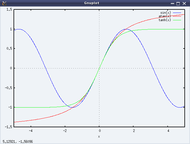
Next is the relation between the normal & the hyperbolic trigo functions.

$ maxima -q
(%i1) sin(%i * x);
(%o1)                            %i sinh(x)
(%i2) cos(%i * x);
(%o2)                              cosh(x)
(%i3) tan(%i * x);
(%o3)                            %i tanh(x)
(%i4) quit();

By enabling the option variable halfangles, many half angle identities, come into play. To be specific, sin(x/2) gets further simplified in (0, 2 * %pi) range, cos(x/2) gets further simplified in (-%pi/2, %pi/2) range. Check out the differences, before and after enabling the option variable, along with the range modifications, in the examples below:

$ maxima -q
(%i1) string(2*cos(x/2)^2 - 1); /* No effect */
(%o1)                           2*cos(x/2)^2-1
(%i2) string(cos(x/2)); /* No effect */
(%o2)                              cos(x/2)
(%i3) halfangles:true; /* Enabling half angles */
(%o3)                                true
(%i4) string(2*cos(x/2)^2 - 1); /* Simplified */
(%o4)                               cos(x)
(%i5) string(cos(x/2)); /* Complex expansion for all x */
(%o5)         (-1)^floor((x+%pi)/(2*%pi))*sqrt(cos(x)+1)/sqrt(2)
(%i6) assume(-%pi < x, x < %pi); /* Limiting x values */
(%o6)                        [x > - %pi, x < %pi]
(%i7) string(cos(x/2)); /* Further simplified */
(%o7)                       sqrt(cos(x)+1)/sqrt(2)
(%i8) quit();

Trigonometric Expansions and Simplifications

Trigonometry is full of multiples of angles, sums of angles, products & powers of trigo functions, and the long list of relations between them. Multiples and sums of angles fall into one category. Products and powers of trigo functions in an another category. And its very useful to do conversions from one of these categories to the other one, to crack a range of simple to complex problems, catering to basic hobby science to quantum mechanics. trigexpand() does the conversion from “multiples & sums of angles” to “products & powers of trigo functions”. trigreduce() does exactly the opposite. Here’s goes a small demo:

$ maxima -q
(%i1) trigexpand(sin(2*x));
(%o1)                           2 cos(x) sin(x)
(%i2) trigexpand(sin(x+y)-sin(x-y));
(%o2)                           2 cos(x) sin(y)
(%i3) trigexpand(cos(2*x+y)-cos(2*x-y));
(%o3)                         - 2 sin(2 x) sin(y)
(%i4) trigexpand(%o3);
(%o4)                      - 4 cos(x) sin(x) sin(y)
(%i5) string(trigreduce(%o4));
(%o5)                  -2*(cos(y-2*x)/2-cos(y+2*x)/2)
(%i6) string(trigsimp(%o5));
(%o6)                       cos(y+2*x)-cos(y-2*x)
(%i7) string(trigexpand(cos(2*x)));
(%o7)                         cos(x)^2-sin(x)^2
(%i8) string(trigexpand(cos(2*x) + 2*sin(x)^2));
(%o8)                         sin(x)^2+cos(x)^2
(%i9) trigsimp(trigexpand(cos(2*x) + 2*sin(x)^2));
(%o9)                                 1
(%i10) quit();

In %o5 above, you might have noted that the 2’s could have been cancelled for further simplification. But that is not the job of trigreduce(), and for that we have to apply the trigsimp() function as shown in %i6. In fact, many other trigonometric identities based simplification are achieved using trigsimp(). Check out the %i7 to %o9 sequences for another such example.

Eighteenth Article >>

   Send article as PDF   

Kernel Window: Peeping through /proc

This sixteenth article, which is part of the series on Linux device drivers, demonstrates the creation and usage of files under the /proc virtual file-system.

<< Fifteenth Article

Useful kernel windows

After many months, Shweta and Pugs got together for a peaceful technical romancing. All through, we have been using all kinds of kernel windows especially through the /proc virtual file-system (using cat), to help us out in decoding the various nitty-gritties of Linux device drivers. Here’s a non-exhaustive summary listing:

  • /proc/modules – Listing of all the dynamically loaded modules
  • /proc/devices – Listing of all the registered character and block major numbers
  • /proc/iomem – Listing of on-system physical RAM & bus device addresses
  • /proc/ioports – Listing of on-system I/O port addresses (specially for x86 systems)
  • /proc/interrupts – Listing of all the registered interrupt request numbers
  • /proc/softirqs – Listing of all the registered soft irqs
  • /proc/kallsyms – Listing of all the running kernel symbols, including from loaded modules
  • /proc/partitions – Listing of currently connected block devices & their partitions
  • /proc/filesystems – Listing of currently active file-system drivers
  • /proc/swaps – Listing of currently active swaps
  • /proc/cpuinfo – Information about the CPU(s) on the system
  • /proc/meminfo – Information about the memory on the system, viz. RAM, swap, …

Custom kernel windows

“Yes, these have been really helpful in understanding and debugging the Linux device drivers. But is it possible for us to also provide some help? Yes, I mean can we create one such kernel window through /proc?”, questioned Shweta.

“Why one? As many as you want. And that’s simple – just use the right set of APIs and there you go.”

“For you every thing is simple.”

“No yaar, this is seriously simple”, smiled Pugs. “Just watch out, me creating one for you.”

And in jiffies, Pugs created the proc_window.c file below (including the changes, which has taken place in kernel v3.10 and v4.3):

#include <linux/module.h>
#include <linux/kernel.h>
#include <linux/version.h>
#if (LINUX_VERSION_CODE < KERNEL_VERSION(3,10,0))
#else
#include <linux/fs.h>
#include <linux/seq_file.h>
#endif
#include <linux/proc_fs.h>
#include <linux/jiffies.h>
#include <linux/uaccess.h>

#if (LINUX_VERSION_CODE < KERNEL_VERSION(3,10,0))
#define STR_PRINTF_RET(len, str, args...) len += sprintf(page + len, str, ## args)
#elif (LINUX_VERSION_CODE < KERNEL_VERSION(4,3,0))
#define STR_PRINTF_RET(len, str, args...) len += seq_printf(m, str, ## args)
#else
#define STR_PRINTF_RET(len, str, args...) seq_printf(m, str, ## args)
#endif

static struct proc_dir_entry *parent, *file, *link;
static int state = 0;

#if (LINUX_VERSION_CODE < KERNEL_VERSION(3,10,0))
static int time_read(char *page, char **start, off_t off, int count, int *eof,
	void *data)
#else
static int time_read(struct seq_file *m, void *v)
#endif
{
	int len = 0, val;
	unsigned long act_jiffies;

	STR_PRINTF_RET(len, "state = %d\n", state);
	act_jiffies = jiffies - INITIAL_JIFFIES;
	val = jiffies_to_msecs(act_jiffies);
	switch (state)
	{
		case 0:
			STR_PRINTF_RET(len, "time = %ld jiffies\n", act_jiffies);
			break;
		case 1:
			STR_PRINTF_RET(len, "time = %d msecs\n", val);
			break;
		case 2:
			STR_PRINTF_RET(len, "time = %ds %dms\n",
					val / 1000, val % 1000);
			break;
		case 3:
			val /= 1000;
			STR_PRINTF_RET(len, "time = %02d:%02d:%02d\n",
					val / 3600, (val / 60) % 60, val % 60);
			break;
		default:
			STR_PRINTF_RET(len, "\n");
			break;
	}

	return len;
}
#if (LINUX_VERSION_CODE < KERNEL_VERSION(3,10,0))
static int time_write(struct file *file, const char __user *buffer,
	unsigned long count, void *data)
#else
static ssize_t time_write(struct file *file, const char __user *buffer,
	size_t count, loff_t *off)
#endif
{
	char kbuf[2];

	if (count > 2)
		return count;
	if (copy_from_user(kbuf, buffer, count))
	{
		return -EFAULT;
	}
	if ((count == 2) && (kbuf[1] != '\n'))
		return count;
	if ((kbuf[0] < '0') || ('9' < kbuf[0]))
		return count;
	state = kbuf[0] - '0';
	return count;
}
#if (LINUX_VERSION_CODE < KERNEL_VERSION(3,10,0))
#else
static int time_open(struct inode *inode, struct file *file)
{
	return single_open(file, time_read, NULL);
}

static struct file_operations fops =
{
	.owner = THIS_MODULE,
	.open = time_open,
	.read = seq_read,
	.write = time_write
};
#endif

static int __init proc_win_init(void)
{
	if ((parent = proc_mkdir("anil", NULL)) == NULL)
	{
		return -1;
	}
#if (LINUX_VERSION_CODE < KERNEL_VERSION(3,10,0))
	if ((file = create_proc_entry("rel_time", 0666, parent)) == NULL)
#else
	if ((file = proc_create("rel_time", 0666, parent, &fops)) == NULL)
#endif
	{
		remove_proc_entry("anil", NULL);
		return -1;
	}
#if (LINUX_VERSION_CODE < KERNEL_VERSION(3,10,0))
	file->read_proc = time_read;
	file->write_proc = time_write;
#endif
	if ((link = proc_symlink("rel_time_l", parent, "rel_time")) == NULL)
	{
		remove_proc_entry("rel_time", parent);
		remove_proc_entry("anil", NULL);
		return -1;
	}
#if (LINUX_VERSION_CODE < KERNEL_VERSION(3,10,0))
	link->uid = 0;
	link->gid = 100;
#else
	proc_set_user(link, KUIDT_INIT(0), KGIDT_INIT(100));
#endif
	return 0;
}

static void __exit proc_win_exit(void)
{
	remove_proc_entry("rel_time_l", parent);
	remove_proc_entry("rel_time", parent);
	remove_proc_entry("anil", NULL);
}

module_init(proc_win_init);
module_exit(proc_win_exit);

MODULE_LICENSE("GPL");
MODULE_AUTHOR("Anil Kumar Pugalia <email@sarika-pugs.com>");
MODULE_DESCRIPTION("Kernel window /proc Demonstration Driver");

And then Pugs did the following steps:

  • Built the driver (proc_window.ko file) using the usual driver’s Makefile.
  • Loaded the driver using insmod.
  • Showed various experiments using the newly created proc windows. (Refer to Figure 28.)
  • And finally, unloaded the driver using rmmod.
Figure 28: Peeping through /proc

Figure 28: Peeping through /proc

Demystifying the details

Starting from the constructor proc_win_init(), three proc entries are created:

  • Directory anil under /proc (i.e. NULL parent) with default permissions 0755, using proc_mkdir()
  • Regular file rel_time under the above directory anil with permissions 0666, using create_proc_entry() or proc_create() (since kernel v3.10)
  • Soft link rel_time_l to the above file rel_time under the same directory anil, using proc_symlink()

The corresponding removal of these three is achieved using remove_proc_entry() in the destructor proc_win_exit(), in chronological reverse order.

For every entry created under /proc, a corresponding struct proc_dir_entry is created. After which many of its fields could be further updated as needed:

  • mode – Permissions of the file
  • uid – User ID of the file
  • gid – Group ID of the file

Since kernel v3.10, specific API proc_set_user() has been provided to update the uid & gid, instead of directly modifying the fields.

Additionally, for a regular file, the following two function pointers for read and write over the file could be provided, respectively:

  • int (*read_proc)(char *page, char **start, off_t off, int count, int *eof, void *data)
  • int (*write_proc)(struct file *file, const char __user *buffer, unsigned long count, void *data)

Again, since kernel v3.10, the read & write fields of struct file_operations are to be used respectively, instead of the above two.

write_proc() is very similar to the character device file operation write. And the above code implementation, lets the user to write a digit from 0 to 9, and accordingly sets the internal state.

read_proc() in the above code implementation provides the current state and the time since the system has been booted up in different units based on the current state. These are, jiffies in state 0; milliseconds in state 1; seconds & milliseconds in state 2; hours : minutes : seconds in state 3; and <not implemented> in other states. And to check the computation accuracy, Figure 29 highlights the system up time in the output of top. read_proc()‘s page parameter is a page-sized buffer, typically to be filled up with count bytes from offset off. But more often than not (because of small content), just page is filled up, ignoring all other parameters. Since kernel v3.10, the read logic has to be implemented through something called a sequence file, which is implemented by specifying the pre-defined seq_read() function for the file operation read, and then by providing the above logic in the sequence file’s read function through the file operation open using single_open().

Figure 29: Comparison with top's output

Figure 29: Comparison with top’s output

All the /proc related structure definitions and function declarations are available through <linux/proc_fs.h>. The sequence file related stuff (since kernel v3.10) are available through <linux/seq_file.h>. And the jiffies related function declarations and macro definitions are in <linux/jiffies.h>. On a special note, the actual jiffies are being calculated by subtracting INITIAL_JIFFIES, as on boot-up, jiffies is initialized to INITIAL_JIFFIES instead of zero.

Summing up

“Hey Pugs!!! Why did you create the folder named as anil? Who is this Anil? You could have used my name or may be yours.” suggested Shweta. “Ha!! That’s a surprise. My real name is Anil only. It is just that everyone in college knows me only as Pugs”, smiled Pugs. Watch out for further technical romancing of Pugs aka Anil.

Seventeenth Article >>

Notes

  1. One of the powerful usage of creating our own proc window is for customized debugging by querying. A simple but cool modification of the above driver, could be instead of getting the jiffies, it could read / write hardware registers.
   Send article as PDF   

Polynomials in Maxima

This sixteenth article of the mathematical journey through open source, demonstrates the polynomial manipulations using Maxima.

<< Fifteenth Article

Polynomials have fascinated mathematicians since ages. Moreover, because of wide variety of their applications, ranging from basic algebra to puzzles to various sciences. Here, we are going to look at some of the polynomial manipulation functions provided by Maxima, and a couple of real world applications using some of them.

Fundamental polynomial operations

Let’s start with a demonstration of the fundamental polynomial operations, like addition, subtraction, multiplication, division. In all these, whenever needed,we’ll use expand() to expand the polynomials, and string() to display the polynomials in a flattened notation.

$ maxima -q
(%i1) p1: x^2 - y^2 + y$
(%i2) p2: -x^2 - y^2 + x$
(%i3) p3: (x + y)^2$
(%i4) string(p1 + p2);
(%o4)                             -2*y^2+y+x
(%i5) string(p1 + p2 + p3);
(%o5)                          (y+x)^2-2*y^2+y+x
(%i6) string(expand(p1 + p2 + p3));
(%o6)                         -y^2+2*x*y+y+x^2+x
(%i7) string(expand(p3 - p1));
(%o7)                            2*y^2+2*x*y-y
(%i8) string(expand(p1 * p2));
(%o8)                   y^4-y^3-x*y^2-x^2*y+x*y-x^4+x^3
(%i9) string(p1 / p2);
(%o9)                     (-y^2+y+x^2)/(-y^2-x^2+x)
(%i10) string(divide(p1, p2));
(%o10)                           [1,y+2*x^2-x]
(%i11) string(divide(x^2 - y^2, x + y));
(%o11)                              [x-y,0]
(%i12) quit();

Note that the / operator just places the polynomials as a fraction, rather then dividing them. And the function divide() actually divides the first polynomial by the second one, yielding a list with the quotient and the remainder of the division. If the division needs to be with respect to a particular variable, that can be passed as the third argument to divide. Check out the variation below, to understand what it means:

$ maxima -q
(%i1) string(divide(x^2 - y^2 + y, x + y, x));
(%o1)                              [x-y,y]
(%i2) string(divide(x^2 - y^2 + y, x + y, y));
(%o2)                            [-y+x+1,-x]
(%i3) quit();

Coefficients of a polynomial

Extracting the coefficients of a polynomial is another basic and common requirement for polynomial manipulations. Maxima provides two slightly different mechanisms. First one, just finds the coefficient of a given variable or its some power, using coeff(). Second one, segregates a polynomial into the coefficient of a given variable or its power, and the remaining terms, using bothcoef().

$ maxima -q
(%i1) string(bothcoef(expand(x^2 - y^2 + (x + y)^2), x^2));
(%o1)                             [2,2*x*y]
(%i2) string(bothcoef(expand(x^2 - y^2 + (x + y)^2), x));
(%o2)                            [2*y,2*x^2]
(%i3) string(bothcoef(expand(x^2 - y^2 + (x + y)^2), y^2));
(%o3)                          [0,2*x*y+2*x^2]
(%i4) string(bothcoef(expand(x^2 - y^2 + (x + y)^2), y));
(%o4)                            [2*x,2*x^2]
(%i5) string(coeff(expand((x + 2 * y)^50), x^20));
(%o5)                   50604606318512743383040*y^30
(%i6) string(coeff(expand((a + b + c + d)^4), a^3));
(%o6)                            4*d+4*c+4*b
(%i7) quit();

Polynomial fractions

Calculating the greatest common divisor (GCD) is one of the very useful operations to simply fractions of polynomials. Other common requirements are extracting the numerator, the denominator, and the highest power. Here goes the function demonstrations for all of these:

$ maxima -q
(%i1) gcd(x^3 + 3*x^2 + 3*x + 1, x^2 + 3*x + 2);
(%o1)                              x + 1
(%i2) string(ezgcd(x^3 + 3*x^2 + 3*x + 1, x^2 + 3*x + 2));
(%o2)                       [x+1,x^2+2*x+1,x+2]
(%i3) string(denom((x + 1)^-3 * (1 - x)^2));
(%o3)                             (x+1)^3
(%i4) string(num((x + 1)^-3 * (1 - x)^2));
(%o4)                             (1-x)^2
(%i5) hipow(expand((x + 1)^3 + (1 - x)^3), x);
(%o5)                                2
(%i6) quit();

Note that the ezgcd() function lists out the remainder polynomials, along with the GCD.

Polynomial fractions could be differentiated using the powerful ratdiff().

$ maxima -q
(%i1) string(ratdiff((x + 1)^-1 * (1 - x)^2, x));
(%o1)                     (x^2+2*x-3)/(x^2+2*x+1)
(%i2) string(ratdiff(1 / (x + 1), x));
(%o2)                         -1/(x^2+2*x+1)
(%i3) string(ratdiff((x^2 - 1) / (x + 1), x));
(%o3)                                1
(%i4) quit();

And, ratsubst() is a powerful expression substitution function, with intelligence. It would dig into the expression to simplify complicated expressions, including trigonometric ones. Check out the %i5, for one of its powerful application. ratsubst(<new>, <old>, <expr>) replaces the <old> expression by the <new> expression in the complete expression <expr>.

$ maxima -q
(%i1) string(ratsubst(u, x^2, x^3 + 3*x^2 + 3*x + 1));
(%o1)                          (u+3)*x+3*u+1
(%i2) string(ratsubst(u, x^2, (x+1)^3));
(%o2)                          (u+3)*x+3*u+1
(%i3) string(ratsubst(u, x^2, (x+1)^4));
(%o3)                       (4*u+4)*x+u^2+6*u+1
(%i4) string(ratsubst(u, x - 1, x^4 - 2*x^2 + 1));
(%o4)                         u^4+4*u^3+4*u^2
(%i5) string(ratsubst(sin(x)^2, 1 - cos(x)^2, cos(x)^4 - 2*cos(x)^2 + 1));
(%o5)                            sin(x)^4
(%i5) quit();

Variable eliminations & equation solving

Very often, we come across N sets of equations in M sets of unknowns, where M >= N. If M = N, then most likely there exists a unique solution. However, if M > N, then there may be many possible solutions, but with some constraints. And in such case, it would be helpful to deduce some simpler set of expressions. This can be achieved using eliminate() of Maxima. Let’s have two polynomial expressions in 3 variables x, y, z to demonstrate the same.

$ maxima -q
(%i1) p1: x^2 + 2*x*y + z^2$
(%i2) p2: x + y + z$
(%i3) string(eliminate([p1, p2], [x]));
(%o3)                            [2*z^2-y^2]
(%i4) string(eliminate([p1, p2], [y]));
(%o4)                         [-z^2+2*x*z+x^2]
(%i5) string(eliminate([p1, p2], [z]));
(%o5)                         [y^2+4*x*y+2*x^2]
(%i6) quit();

Note that in all the above polynomial expressions, the expressions are assumed to be equated to zero. A beautiful application of the above is solving recurrence relations. Let’s say we have a non-linear equation given by Yn+1 = r * Yn * (1 – Yn). And, we want to solve it for a scenario that as n tends to infinity, the value of Y oscillates between two distinct values. This means that Yn+2 = Yn. Hence, we would have two expressions with three unknowns to solve with, namely:

  1. Yn+1 = r * Yn * (1 – Yn)
  2. Yn = r * Yn+1 * (1 – Yn+1)

So, representing Yn+1 with yn1 and Yn by yn, we may use solve() to solve for yn & yn1 in terms of r. But, if rather we want to get a feel of the equation which pops up, in terms of yn, we would have to use eliminate() to eliminate yn1.

$ maxima -q
(%i1) p1: yn1 = r * yn * (1 - yn)$
(%i2) p2: yn = r * yn1 * (1 - yn1)$
(%i3) string(eliminate([p1, p2], [yn1]));
(%o3)          [yn*(r^3*yn^3-2*r^3*yn^2+(r^3+r^2)*yn-r^2+1)]
(%i4) string(solve([p1, p2], [yn, yn1])); /* Just to show the solution */
(%o4) [[yn = (r-1)/r,yn1 = (r-1)/r],
    [yn = -(sqrt(r^2-2*r-3)-r-1)/(2*r),yn1 = (sqrt(r-3)*sqrt(r+1)+r+1)/(2*r)],
    [yn = (sqrt(r^2-2*r-3)+r+1)/(2*r),yn1 = -(sqrt(r-3)*sqrt(r+1)-r-1)/(2*r)],
    [yn = 0,yn1 = 0]]
(%i5) quit()

Seventeenth Article >>

   Send article as PDF   

Disk on RAM: Playing destructively

This fifteenth article, which is part of the series on Linux device drivers, experiments with a dummy hard disk on RAM to demonstrate the block drivers.

<< Fourteenth Article

Play first, rules later

After a delicious lunch, theory makes audience sleepy. So, let’s start with the code itself. Code demonstrated is available at dor_code.tar.bz2. This tar ball contains 3 ‘C’ source files, 2 ‘C’ headers, and a Makefile. As usual, executing make will build the ‘disk on ram’ driver (dor.ko) – this time combining the 3 ‘C’ files. Check out the Makefile to see how. make clean would do the usual clean of the built stuff.

Once built, the following are the experimenting steps (Refer to Figures 25, 26, 27):

  • Load the driver dor.ko using insmod. This would create the block device files representing the disk on 512 KibiBytes (KiB) of RAM, with 3 primary and 3 logical partitions.
  • Checkout the automatically created block device files (/dev/rb*). /dev/rb is the entire disk of 512 KiB size. rb1, rb2, rb3 are the primary partitions with rb2 being the extended partition and containing the 3 logical partitions rb5, rb6, rb7.
  • Read the entire disk (/dev/rb) using the disk dump utility dd.
  • Zero out the first sector of the disk’s first partition (/dev/rb1) again using dd.
  • Write some text into the disk’s first partition (/dev/rb1) using cat.
  • Display the initial contents of the first partition (/dev/rb1) using the xxd utility. See Figure 26 for the xxd output.
  • Display the partition info for the disk using fdisk. See Figure 27 for the fdisk output.
  • (Quick) Format the third primary partition (/dev/rb3) as vfat filesystem (like your pen drive), using mkfs.vfat (Figure 27).
  • Mount the newly formatted partition using mount, say at /mnt (Figure 27).
  • Disk usage utility df would now show this partition mounted at /mnt (Figure 27). You may go ahead and store your files there. But, please remember that these partitions are all on a disk on RAM, and so non-persistent. Hence,
  • Unloading the driver using ‘rmmod dor‘ would vanish everything. Though the partition needs to be unmounted using ‘umount /mnt‘ before doing that.

Please note that all the above experimenting steps need to be executed with root privileges.

Figure 25: Playing with 'Disk on RAM' driver

Figure 25: Playing with ‘Disk on RAM’ driver

Figure 26: xxd showing the initial data on the first partition (/dev/rb1)

Figure 26: xxd showing the initial data on the first partition (/dev/rb1)

Figure 27: Formatting the third partition (/dev/rb3)

Figure 27: Formatting the third partition (/dev/rb3)

Now, let’s learn the rules

We have just now played around with the disk on RAM but without actually knowing the rules, i.e. the internal details of the game. So, let’s dig into the nitty-gritties to decode the rules. Each of the three .c files represent a specific part of the driver. ram_device.c and ram_device.h abstract the underlying RAM operations like vmalloc/vfree, memcpy, etc, providing disk operation APIs like init/cleanup, read/write, etc. partition.c and partition.h provide the functionality to emulate the various partition tables on the disk on RAM. Recall the pre-lunch session (i.e. the previous article) to understand the details of partitioning. The code in this is responsible for the partition information like number, type, size, etc that is shown up on the disk on RAM using fdisk. ram_block.c is the core block driver implementation exposing the disk on RAM as the block device files (/dev/rb*) to the user-space. In other words, the four files ram_device.* and partition.* form the horizontal layer of the device driver and ram_block.c forms the vertical (block) layer of the device driver. So, let’s understand that in detail.

The block driver basics

Conceptually, the block drivers are very similar to character drivers, especially with regards to the following:

  • Usage of device files
  • Major and minor numbers
  • Device file operations
  • Concept of device registration

So, if one already knows character driver implementations, it would be similar to understand the block drivers. Though, they are definitely not identical. The key differences could be listed out as follows:

  • Abstraction for block-oriented versus byte-oriented devices
  • Block drivers are designed to be used by I/O schedulers, for optimal performance. Compare that with character drivers to be used by VFS.
  • Block drivers are designed to be integrated with the Linux’ buffer cache mechanism for efficient data access. Character drivers are pass-through drivers, accessing the hardware directly.

And these trigger the implementation differences. Let’s analyze the key code snippets from ram_block.c, starting at the driver’s constructor rb_init().

First step is to register for a 8-bit (block) major number. And registering for that implicitly means registering for all the 256 8-bit minor numbers associated with that. The function for that is:

int register_blkdev(unsigned int major, const char *name);

major is the major number to be registered. name is a registration label displayed under the kernel window /proc/devices. Interestingly, register_blkdev() tries to allocate & register a freely available major number, when 0 is passed for its first parameter major; and on success, the allocated major number is returned. The corresponding deregistration function is:

void unregister_blkdev(unsigned int major, const char *name);

Both are prototyped in <linux/fs.h>

Second step is to provide the device file operations, through the struct block_device_operations (prototyped in <linux/blkdev.h>) for the registered major number device files. However, these operations are too few compared to the character device file operations, and mostly insignificant. To elaborate, there are no operations even to read and write. That’s surprising. But as we already know that the block drivers need to integrate with the I/O schedulers, the read-write implementation is achieved through something called request queues. So, along with providing the device file operations, the following needs to provided:

  • Request queue for queuing the read/write requests
  • Spin lock associated with the request queue for its concurrent access protection
  • Request function to process the requests queued in the request queue

Also, there is no separate interface for block device file creations, so the following are also provided:

  • Device file name prefix, commonly referred as disk_name (“rb” in the dor driver)
  • Starting minor number for the device files, commonly referred as the first_minor

Finally, two block device-specific things are also provided along with the above, namely:

  • Maximum number of partitions supported for this block device, by specifying the total minors
  • Underlying device size in units of 512-byte sectors, for the logical block access abstraction

All these are registered through the struct gendisk using the function:

void add_disk(struct gendisk *disk);

The corresponding delete function is:

void del_gendisk(struct gendisk *disk);

Prior to add_disk(), the various fields of struct gendisk need to be initialized, either directly or using various macros/functions like set_capacity(). major, first_minor, fops, queue, disk_name are the minimal fields to be initialized directly. And even before the initialization of these fields, the struct gendisk needs to be allocated using the function:

struct gendisk *alloc_disk(int minors);

where minors is the total number of partitions supported for this disk. And the corresponding inverse function would be:

void put_disk(struct gendisk *disk);

All these are prototyped in <linux/genhd.h>.

Request queue and its request processing function

The request queue also needs to be initialized and set up into the struct gendisk, before the add_disk(). The request queue is initialized by calling:

struct request_queue *blk_init_queue(request_fn_proc *, spinlock_t *);

providing the request processing function and the initialized concurrency protection spinlock, as its parameters. The corresponding queue cleanup function is:

void blk_cleanup_queue(struct request_queue *);

The request (processing) function should be defined with the following prototype:

void request_fn(struct request_queue *q);

And it should be coded to fetch a request from its parameter q, say using

struct request *blk_fetch_request(struct request_queue *q);

and then either process it or initiate the processing. Whatever it does, it should be non-blocking, as this request function is called from a non-process context, and also after taking the queue’s spinlock. So, moreover only the functions not releasing or taking the queue’s spinlock should be used within the request function.

A typical request processing as demonstrated by the function rb_request() in ram_block.c is:

while ((req = blk_fetch_request(q)) != NULL) /* Fetching a request */
{
	/* Processing the request: the actual data transfer */
	ret = rb_transfer(req); /* Our custom function */
	/* Informing that the request has been processed with return of ret */
	__blk_end_request_all(req, ret);
}

Request and its processing

rb_transfer() is our key function, which parses a struct request and accordingly does the actual data transfer. The struct request mainly contains the direction of data transfer, starting sector for the data transfer, total number of sectors for the data transfer, and the scatter-gather buffer for data transfer. The various macros to extract these information from the struct request are as follows:

rq_data_dir(req); /* Operation: 0 - read from device; otherwise - write to device */
blk_req_pos(req); /* Starting sector to process */
blk_req_sectors(req); /* Total sectors to process */
rq_for_each_segment(bv, req, iter) /* Iterator to extract individual buffers */

rq_for_each_segment() is the special one which iterates over the struct request (req) using iter, and extracting the individual buffer information into the struct bio_vec (bv: basic input/output vector) on each iteration. And, then on each extraction, the appropriate data transfer is done, based on the operation type, invoking one of the following APIs from ram_device.c:

void ramdevice_write(sector_t sector_off, u8 *buffer, unsigned int sectors);
void ramdevice_read(sector_t sector_off, u8 *buffer, unsigned int sectors);

Check out the complete code of rb_transfer() in ram_block.c

Summing up

“With that, we have actually learnt the beautiful block drivers by traversing through the design of a hard disk, and playing around with partitioning, formatting, and various other raw operations on a hard disk. Thanks for your patient listening. Now, the session is open for questions. Or, you may post your queries as comments, below.”

Sixteenth Article >>

   Send article as PDF   

Expression Simplification using Maxima

This fifteenth article of the mathematical journey through open source, demonstrates the various techniques of expression simplification using Maxima.

<< Fourteenth Article

Expression simplification can be done in a variety of ways. Let’s start with the simple ones, and then move onto more powerful ones.

Real number simplification

A simple simplification is to convert a given number into a rational number using ratsimp(). Below follows the demonstration.

$ maxima -q
(%i1) ratsimp(9);
(%o1)                                  9
(%i2) ratsimp(10.0);
rat: replaced 10.0 by 10/1 = 10.0
(%o2)                                 10
(%i3) string(ratsimp(4.2)); /* string to print it on one line */
rat: replaced 4.2 by 21/5 = 4.2
(%o3)                               21/5
(%i4) string(factor(3.2)); /* string to print it on one line */
rat: replaced 3.2 by 16/5 = 3.2
(%o4)                                2^4/5
(%i5) string(ratsimp(4.3333)); /* string to print it on one line */
rat: replaced 4.3333 by 43333/10000 = 4.3333
(%o5)                            43333/10000
(%i6) string(ratsimp(4.3333333)); /* string to print it on one line */
rat: replaced 4.3333333 by 13/3 = 4.333333333333333
(%o6)                               13/3
(%i7) quit();

Another one is to check whether a number is an integer using askinteger(). And if yes, is it an even or odd number, again using askinteger(). Moreover, asksign() checks for the sign. In case of trying these with unknown variables, Maxima would ask the user the necessary question(s) to deduce the response, and store it for future analysis. For example, askinteger(x) would ask us if x is an integer. And, if we say yes, it can then deduce many more information by itself. Below are some examples:

$ maxima -q
(%i1) askinteger(1);
(%o1)                                 yes
(%i2) askinteger(1.0);
rat: replaced 1.0 by 1/1 = 1.0
(%o2)                                 yes
(%i3) askinteger(1.2);
rat: replaced 1.2 by 6/5 = 1.2
(%o3)                                 no
(%i4) askinteger(-9);
(%o4)                                 yes
(%i5) askinteger(2/3 + 3/4 + 1/6 + 5/12);
(%o5)                                 yes
(%i6) askinteger(-9, even);
(%o6)                                 no
(%i7) askinteger(0, even);
(%o7)                                 yes
(%i8) properties(x);
(%o8)                                []
(%i9) askinteger(x);
Is x an integer?
yes; /* This is our response */
(%o9)                                 yes
(%i10) askinteger(x + 9);
(%o10)                                 yes
(%i11) askinteger(2 * x, even);
(%o11)                                yes
(%i12) askinteger(2 * x + 1, even);
(%o12)                                no
(%i13) askinteger(x, even);
Is x an even number?
n; /* This is our response */
(%o13)                                no
(%i14) askinteger(x, odd);
(%o14)                                yes
(%i15) askinteger(x^3 - (x + 1)^2, even);
(%o15)                                no
(%i16) properties(x);
(%o16)          [database info, kind(x, integer), kind(x, odd)]
(%i17) asksign((-1)^x);
(%o17)                                neg
(%i18) asksign((-1)^(x+1));
(%o18)                                pos
(%i19) asksign((-1)^x+1);
(%o19)                               zero
(%i20) quit();

Maxima simplification uses the concept of properties of symbols. As an example, note the properties of x in the above demonstration at %i8 and %i16.

Complex number simplification

Complex numbers have two common useful forms, namely the exponential and the circular (with sine & cosine) forms. demoivre() converts the exponential to circular form and exponentialize() does the other way round. Using expand() along with them, can simplify complicated looking expressions. Here goes few examples:

$ maxima -q
(%i1) string(demoivre(exp(%i*x^2))); /* %i is sqrt(-1) */
(%o1)                       %i*sin(x^2)+cos(x^2)
(%i2) string(exponentialize(a*(cos(t)))); /* %i is sqrt(-1) */
(%o2)                    a*(%e^(%i*t)+%e^-(%i*t))/2
(%i3) string(expand(exponentialize(a*(cos(t)+%i*sin(t))))); /* %i is sqrt(-1) */
(%o3)                            a*%e^(%i*t)
(%i4) quit();

Expansions and Reductions

As already seen in the previous article, expand() expands an expression completely, by default. However, it can be controlled by specifying the maximum power to which to expand for both the numerator and the denominator, respectively. Using factor() can compact the expanded expressions. Moreover, in many cases, we would like to expand it only with respect to only some variable(s). Say, (x + a + b)^2 should be expanded with respect to x. expandwrt() is meant exactly for that. One example of each of these is shown below.

$ maxima -q
(%i1) string(expand(((x+1)^2-x^2)/(x+1)^2, 2, 0));
(%o1)                      2*x/(x+1)^2+1/(x+1)^2
(%i2) string(factor(((x+1)^2-x^2)/(x+1)^2));
(%o2)                           (2*x+1)/(x+1)^2
(%i3) string(expandwrt((x+a+b)^2,x));
(%o3)                      x^2+2*(b+a)*x+(b+a)^2
(%i4) quit();

Expressions containing logs, exponentials, radicals (powers) can be simplified using radcan(). Rule based simplifications can be achieved using sequential comparative simplification function scsim(). Both of these call for a few examples.

$ maxima -q
(%i1) string(radcan(exp(5 * log(x) + log(3 * exp(log(y) / 4)))));
(%o1)                          3*x^5*y^(1/4)
(%i2) radcan((log(2*x+2*x^2)-log(x))/(log(1+1/x)+log(2*x)));
(%o2)                                1
(%i3) expr: a^2 + b^2 + c^2$
(%i4) eq1: a^2 + 2*a*b + b^2 = 4$
(%i5) eq2: a * b = 6$
(%i6) string(scsimp(expr, eq1, eq2));
(%o6)                              c^2-8
(%i7) quit();

Unlike Octave, Maxima by default doesn’t evaluate its expressions, it only simplifies. What it means is that expressions with integers like cos(1), exp(2), sqrt(3), etc. may remain as is in the most simplified form, instead of evaluating to their respective float numerical values. In such cases, we may force the evaluation by passing the option numer. Similar evaluation can be achieved for predicates, using pred.

$ maxima -q
(%i1) cos(1);
(%o1)                             cos(1)
(%i2) cos(1), numer;
(%o2)                        .5403023058681398
(%i3) sqrt(7);
(%o3)                             sqrt(7)
(%i4) sqrt(7), numer;
(%o4)                        2.645751311064591
(%i4) 1 + 2 > 9;
(%o4)                              3 > 9
(%i5) 1 + 2 > 9, pred;
(%o5)                              false
(%i6) string(%e^%pi < %pi^%e); /* string to print it on one line */
(%o6)                         %e^%pi < %pi^%e
(%i7) %e^%pi < %pi^%e, pred;
(%o7)                              false
(%i8) quit();

Summation Simplifications

Symbolical representation and manipulations of summations can be beautifully achieved using sum() and the option simpsum. Check out the code execution below:

$ maxima -q
(%i1) sum(a * i, i, 1, 5);
(%o1)                                15 a
(%i2) sum(a, i, 1, 5);
(%o2)                                 5 a
(%i3) sum(a * i, i, 1, n);
                                      n
                                     ====
                                     \
(%o3)                              a  >    i
                                     /
                                     ====
                                     i = 1
(%i4) simpsum: true$ /* Enable simplification of summations */
(%i5) string(sum(a * i, i, 1, n)); /* string to print it on one line */
(%o5)                            a*(n^2+n)/2
(%i6) string(sum(i^2 - i, i, 1, n) + sum(j, j, 1, n));
(%o6)                         (2*n^3+3*n^2+n)/6
(%i7) string(factor(sum(i^2 - i, i, 1, n) + sum(j, j, 1, n)));
(%o7)                         n*(n+1)*(2*n+1)/6
(%i8) quit();

Sixteenth Article >>

   Send article as PDF   

Understanding the Partitions: A dive inside the hard disk

This fourteenth article, which is part of the series on Linux device drivers, takes you for a walk inside a hard disk.

<< Thirteenth Article

Hard disk design

“Doesn’t it sound like a mechanical engineering subject: Design of hard disk?”, questioned Shweta. “Yes, it does. But understanding it gets us an insight into its programming aspect”, reasoned Pugs while waiting for the commencement of the seminar on storage systems.

Figure 23: Partition listing by fdisk

Figure 23: Partition listing by fdisk

The seminar started with a few hard disks in the presenter’s hand and then a dive down into her system showing the output of fdisk -l, as shown in Figure 23. The first line shows the hard disk size in human friendly format and in bytes. The second line mentions the number of logical heads, logical sectors per track, and the actual number of cylinders on the disk – these together are referred as the geometry of the disk. The 255 heads indicating the number of platters or disks, as one read-write head is needed per disk. Let’s number them say D1, D2, …, D255. Now, each disk would have the same number of concentric circular tracks, starting from outside to inside. In the above case there are 60801 such tracks per disk. Let’s number them say T1, T2, …, T60801. And a particular track number from all the disks forms a cylinder of the same number. For example, tracks T2 from D1, D2, …, D255 will all together form the cylinder C2. Now, each track has the same number of logical sectors – 63 in our case, say S1, S2, …, S63. And each sector is typically 512 bytes. Given this data, one can actually compute the total usable hard disk size, using the following formula:

Usable hard disk size in bytes = (Number of heads or disks) * (Number of tracks per disk) * (Number of sectors per track) * (Number of bytes per sector, i.e. sector size).

For the disk under consideration it would be: 255 * 60801 * 63 * 512 bytes = 500105249280 bytes. Note that this number may be slightly less than the actual hard disk – 500107862016 bytes in our case. The reason for that is that the formula doesn’t consider the bytes in last partial or incomplete cylinder. And the primary reason for that is the difference between today’s technology of organizing the actual physical disk geometry and the traditional geometry representation using heads, cylinders, sectors. Note that in the fdisk output, we referred to the heads, and sectors per track as logical not the actual one. One may ask, if today’s disks doesn’t have such physical geometry concepts, then why to still maintain that and represent them in more of logical form. The main reason is to be able to continue with same concepts of partitioning and be able to maintain the same partition table formats especially for the most prevalent DOS type partition tables, which heavily depend on this simplistic geometry. Note the computation of cylinder size (255 heads * 63 sectors / track * 512 bytes / sector = 8225280 bytes) in the third line and then the demarcation of partitions in units of complete cylinders.

DOS type partition tables

This brings us to the next important topic of understanding the DOS type partition tables. But in the first place, what is a partition and rather why to even partition? A hard disk can be divided into one more logical disks, each of which is called a partition. And this is useful for organizing different types of data separately. For example, different operating system data, user data, temporary data, etc. So, partitions are basically logical divisions and hence need to be maintained through some meta data, which is the partition table. A DOS type partition table contains 4 partition entries, each being a 16-byte entry. And each of these entries can be depicted by the following ‘C’ structure:

typedef struct
{
	unsigned char boot_type; // 0x00 - Inactive; 0x80 - Active (Bootable)
	unsigned char start_head;
	unsigned char start_sec:6;
	unsigned char start_cyl_hi:2;
	unsigned char start_cyl;
	unsigned char part_type;
	unsigned char end_head;
	unsigned char end_sec:6;
	unsigned char end_cyl_hi:2;
	unsigned char end_cyl;
	unsigned int abs_start_sec;
	unsigned int sec_in_part;
} PartEntry;

And this partition table followed by the two-byte signature 0xAA55 resides at the end of hard disk’s first sector, commonly known as Master Boot Record or MBR (in short). Hence, the starting offset of this partition table within the MBR is 512 – (4 * 16 + 2) = 446. Also, a 4-byte disk signature is placed at the offset 440. The remaining top 440 bytes of the MBR are typically used to place the first piece of boot code, that is loaded by the BIOS to boot up the system from the disk. Listing of part_info.c contains these various defines, and the code for parsing and printing a formatted output of the partition table of one’s hard disk.

From the partition table entry structure, it could be noted that the start and end cylinder fields are only 10 bits long, thus allowing a maximum of 1023 cylinders only. However, for today’s huge hard disks, this size is no way sufficient. And hence in overflow cases, the corresponding <head, cylinder, sector> triplet in the partition table entry is set to the maximum value, and the actual value is computed using the last two fields: the absolute start sector number (abs_start_sec) and the number of sectors in this partition (sec_in_part). Listing of part_info.c contains the code for this as well.

#include <stdio.h>
#include <sys/types.h>
#include <sys/stat.h>
#include <fcntl.h>
#include <unistd.h>

#define MBR_DISK_SIGNATURE_OFFSET 440
#define PARTITION_ENTRY_SIZE 16 // sizeof(PartEntry)
#define PARTITION_TABLE_SIZE (4 * PARTITION_ENTRY_SIZE)

typedef struct
{
	unsigned char boot_type; // 0x00 - Inactive; 0x80 - Active (Bootable)
	unsigned char start_head;
	unsigned char start_sec:6;
	unsigned char start_cyl_hi:2;
	unsigned char start_cyl;
	unsigned char part_type;
	unsigned char end_head;
	unsigned char end_sec:6;
	unsigned char end_cyl_hi:2;
	unsigned char end_cyl;
	unsigned int abs_start_sec;
	unsigned int sec_in_part;
} PartEntry;

typedef struct
{
	unsigned char boot_code[MBR_DISK_SIGNATURE_OFFSET];
	unsigned int disk_signature;
	unsigned short pad;
	unsigned char pt[PARTITION_TABLE_SIZE];
	unsigned short signature;
} MBR;

void print_computed(unsigned int sector)
{
	unsigned int heads, cyls, tracks, sectors;

	sectors = sector % 63 + 1 /* As indexed from 1 */;
	tracks = sector / 63;
	cyls = tracks / 255 + 1 /* As indexed from 1 */;
	heads = tracks % 255;
	printf("(%3d/%5d/%1d)", heads, cyls, sectors);
}

int main(int argc, char *argv[])
{
	char *dev_file = "/dev/sda";
	int fd, i, rd_val;
	MBR m;
	PartEntry *p = (PartEntry *)(m.pt);

	if (argc == 2)
	{
		dev_file = argv[1];
	}
	if ((fd = open(dev_file, O_RDONLY)) == -1)
	{
		fprintf(stderr, "Failed opening %s: ", dev_file);
		perror("");
		return 1;
	}
	if ((rd_val = read(fd, &m, sizeof(m))) != sizeof(m))
	{
		fprintf(stderr, "Failed reading %s: ", dev_file);
		perror("");
		close(fd);
		return 2;
	}
	close(fd);
	printf("\nDOS type Partition Table of %s:\n", dev_file);
	printf("  B Start (H/C/S)   End (H/C/S) Type  StartSec    TotSec\n");
	for (i = 0; i < 4; i++)
	{
		printf("%d:%d (%3d/%4d/%2d) (%3d/%4d/%2d)  %02X %10d %9d\n",
			i + 1, !!(p[i].boot_type & 0x80),
			p[i].start_head,
			1 + ((p[i].start_cyl_hi << 8) | p[i].start_cyl),
			p[i].start_sec,
			p[i].end_head,
			1 + ((p[i].end_cyl_hi << 8) | p[i].end_cyl),
			p[i].end_sec,
			p[i].part_type,
			p[i].abs_start_sec, p[i].sec_in_part);
	}
	printf("\nRe-computed Partition Table of %s:\n", dev_file);
	printf("  B Start (H/C/S)   End (H/C/S) Type  StartSec    TotSec\n");
	for (i = 0; i < 4; i++)
	{
		printf("%d:%d ", i + 1, !!(p[i].boot_type & 0x80));
		print_computed(p[i].abs_start_sec);
		printf(" ");
		print_computed(p[i].abs_start_sec + p[i].sec_in_part - 1);
		printf(" %02X %10d %9d\n", p[i].part_type,
			p[i].abs_start_sec, p[i].sec_in_part);
	}
	printf("\n");
	return 0;
}

As the above code (part_info.c) is an application, compile it to an executable (./part_info) as follows: gcc part_info.c -o part_info, and then run ./part_info /dev/sda to check out your primary partitioning information on /dev/sda. Figure 24 shows the output of ./part_info on the presenter’s system. Compare it with the fdisk output as shown in figure 23.

Figure 24: Output of ./part_info

Figure 24: Output of ./part_info

Partition types and Boot records

Now as this partition table is hard-coded to have 4 entries, that dictates the maximum number of partitions, we can have, namely 4. These are called primary partitions, each having a type associated with them in their corresponding partition table entry. The various types are typically coined by the various operating system vendors and hence it is a sort of mapping to the various operating systems, for example, DOS, Minix, Linux, Solaris, BSD, FreeBSD, QNX, W95, Novell Netware, etc to be used for/with the particular operating system. However, this is more of ego and formality than a real requirement.

Apart from these, one of the 4 primary partitions can actually be labeled as something referred as an extended partition, and that has a special significance. As name suggests, it is used to further extend the hard disk division, i.e. to have more partitions. These more partitions are referred as logical partitions and are created within the extended partition. Meta data of the logical partitions is maintained in a linked list format, allowing unlimited number of logical partitions, at least theoretically. For that, the first sector of the extended partition, commonly referred to as Boot Record or BR (in short), is used in a similar way as MBR to store (the linked list head of) the partition table for the logical partitions. Subsequent linked list nodes are stored in the first sector of the subsequent logical partitions, referred to as Logical Boot Record or LBR (in short). Each linked list node is a complete 4-entry partition table, though only the first two entries are used – the first for the linked list data, namely, information about the immediate logical partition, and second one as the linked list’s next pointer, pointing to the list of remaining logical partitions.

To compare and understand the primary partitioning details on your system’s hard disk, follow these steps (as root user and hence with care):

  • ./part_info /dev/sda # Displays the partition table on /dev/sda
  • fdisk -l /dev/sda # To display and compare the partition table entries with the above

In case you have multiple hard disks (/dev/sdb, …), or hard disk device file with other names (/dev/hda, …), or an extended partition, you may try ./part_info <device_file_name> on them as well. Trying on an extended partition would give the information about the starting partition table of the logical partitions.

Summing up

“Right now we carefully and selectively played (read only) with our system’s hard disk. Why carefully? As otherwise, we may render our system non-bootable. But no learning is complete without a total exploration. Hence, in our post-lunch session, we would create a dummy disk on RAM and do the destructive explorations.”

Fifteenth Article >>

   Send article as PDF   

Doing Algebra with Maxima

This fourteenth article of the mathematical journey through open source, introduces to doing algebra using Maxima.

<< Thirteenth Article

Maxima is a computer algebra system derived from the earlier Macsyma, which in turn, was written in Lisp.

Algebraic capability of Maxima is the one, which puts it apart from the others. We have worked through basic shell maths, bench calculator bc, and finally the ultra capable octave. But none of them could do algebra with symbols, also referred as symbolic or analytic mathematics. Let’s walk through a few examples to demonstrate what it means.

Getting started

Maxima command line can be started on the shell by typing maxima. -q option to it suppresses the initial welcome message. Typing quit(); on the Maxima command line quits Maxima. Typical Maxima commands shall be terminated either with a semicolon (;) or a dollar ($) – the later suppressing any print from the command. Outputs are numbered and prefaced by %o. Inputs are also numbered, and prefaced by %i. Here are a few factorization examples:

$ maxima -q
(%i1) factor(x^3 - 1);
                                       2
(%o1)                        (x - 1) (x  + x + 1)
(%i2) factor((x + 1)^4);
                                     4
(%o2)                              (x + 1)
(%i3) expand(%o2);
                           4      3      2
(%o3)                     x  + 4 x  + 6 x  + 4 x + 1
(%i4) factor(6!);
                                     4  2
(%o4)                               2  3  5
(%i5) expand(6!);
(%o5)                                 720
(%i6) quit();

factor() and expand() are two complementary functions doing factorization & simplification, respectively. Note the way the powers in the output are printed. For example, 6! is factorized as 24 * 32 * 5. In case, we want the output on a single line, we may use the command string(), which we shall use now onwards. Also, note the usage of output labels as inputs to the commands, namely expand(%o2) in the above example.

Integration and differentiation

Octave has enabled us to do integration and differentiation, but more of definite integrals and differences. Yes, it has indefinite operations for polynomials. But with Maxima, we can just plug in the expressions, as we usually do on our maths notebooks. This is what it means:

$ maxima -q
(%i1) integrate(cos(x),x);
(%o1)                               sin(x)
(%i2) diff(cos(x),x);
(%o2)                              - sin(x)
(%i3) string(integrate(1/(a^2 + x^2)^(3/2),x));
(%o3)                        x/(a^2*sqrt(x^2+a^2))
(%i4) string(diff(log(x), x));
(%o4)                                 1/x
(%i5) y: (x+1)^2$ /* $ suppresses the output */
(%i6) string(diff(y, x));
(%o6)                              2*(x+1)
(%i7) string(integrate(y, x));
(%o7)                            x^3/3+x^2+x
(%i8) quit();

Variable assignments can be done in Maxima using colon (:), as shown in the input %i5, above. There onwards, the variable can be used instead of the original expression, as shown in the inputs %i6 & %i7. Note that the variable assignment assigns the complete symbolic expression, unlike the usual value assignments.

Solving equations

Whether it be linear set of equations, polynomial equations, or for that matter non-linear equations, Maxima can solve most of them with quite ease, and that also in a analytical way. Here are a few common examples: 1) The two solutions of a quadratic equation; 2) Two simultaneous equations in two variables; 3) A non-linear equation with irrational number e. Maxima code demonstration follows:

$ maxima -q
(%i1) string(solve(a*x^2 + b*x + c = 0, x));
(%o1)   [x = -(sqrt(b^2-4*a*c)+b)/(2*a),x = (sqrt(b^2-4*a*c)-b)/(2*a)]
(%i2) string(solve([a*x + b*y = c,d*x + e*y = f],[x, y]));
(%o2)        [[x = -(c*e-b*f)/(b*d-a*e),y = (c*d-a*f)/(b*d-a*e)]]
(%i3) string(solve([exp(x) + 1/exp(x) = a],[x]));
(%o3)      [x = log(a/2-sqrt(a^2-4)/2),x = log(sqrt(a^2-4)/2+a/2)]
(%i8) quit();

Equation solving has been one of the most fascinating as well as challenging tasks for solving mathematical problems, since ages. So, when the computer is there to aid it, we try to go beyond the human limitations. We just saw the well-known formula for the two solutions of a quadratic equation. How about the same for a cubic equation? It looks really complicated and hence we typically don’t use it. But, still you want to see it. Here it goes:

$ maxima -q
(%i1) string(solve(a*x^3 + b*x^2 + c*x + d = 0, x));
(%o1) [x = (-sqrt(3)*%i/2-1/2)*(sqrt(27*a^2*d^2+(4*b^3-18*a*b*c)*d+4*a*c^3-b^2*c^2)/
(2*3^(3/2)*a^2)-(27*a^2*d-9*a*b*c+2*b^3)/(54*a^3))^(1/3)-(sqrt(3)*%i/2-1/2)*(3*a*c-
b^2)/(9*a^2*(sqrt(27*a^2*d^2+(4*b^3-18*a*b*c)*d+4*a*c^3-b^2*c^2)/(2*3^(3/2)*a^2)-
(27*a^2*d-9*a*b*c+2*b^3)/(54*a^3))^(1/3))-b/(3*a),x = (sqrt(3)*%i/2-1/2)*(sqrt(27*
a^2*d^2+(4*b^3-18*a*b*c)*d+4*a*c^3-b^2*c^2)/(2*3^(3/2)*a^2)-(27*a^2*d-9*a*b*c+2*b^3)/
(54*a^3))^(1/3)-(-sqrt(3)*%i/2-1/2)*(3*a*c-b^2)/(9*a^2*(sqrt(27*a^2*d^2+(4*b^3-18*a*
b*c)*d+4*a*c^3-b^2*c^2)/(2*3^(3/2)*a^2)-(27*a^2*d-9*a*b*c+2*b^3)/(54*a^3))^(1/3))-b/
(3*a),x = (sqrt(27*a^2*d^2+(4*b^3-18*a*b*c)*d+4*a*c^3-b^2*c^2)/(2*3^(3/2)*a^2)-(27*
a^2*d-9*a*b*c+2*b^3)/(54*a^3))^(1/3)-(3*a*c-b^2)/(9*a^2*(sqrt(27*a^2*d^2+(4*b^3-18*
a*b*c)*d+4*a*c^3-b^2*c^2)/(2*3^(3/2)*a^2)-(27*a^2*d-9*a*b*c+2*b^3)/(54*a^3))^(1/3))-
b/(3*a)]
(%i2) quit();

And that’s what is the power of Maxima.

Plotting graphs

Along with the algebraic processing, Maxima also supports graph plotting for the algebraic expressions, though we must specify the intervals to plot it. It can do 2-D as well as 3-D plots. The following code shows an example for each of these. And figures 22 & 23 show the respective plots.

$ maxima -q
(%i1) plot2d([sin(x), atan(x), tanh(x)], [x, -5, 5])$
(%i2) plot3d(sin(abs(x) + abs(y))/(abs(x) + abs(y)),[x, -12, 12], [y, -12, 12])$
(%i3) quit();
Figure 22: Output of plot2d()

Figure 22: Output of plot2d()

Figure 23: Output of plot3d()

Figure 23: Output of plot3d()

After this first glimpse of what Maxima can do, we are now ready to move on to detail out the specific topics, like expression simplification, polynomials, etc.

Fifteenth Article >>

   Send article as PDF   

USB Drivers in Linux: Data Transfer to & from USB Devices

This thirteenth article, which is part of the series on Linux device drivers, details out the ultimate step of data transfer to and from a USB device using your first USB driver in Linux – a continuation from the previous two articles.

<< Twelfth Article

USB miscellany

Pugs continued, “To answer your question about how a driver selectively registers or skips a particular interface of a USB device, you need to understand the significance of the return value of probe() callback.” Note that the USB core would invoke probe for all the interfaces of a detected device, except the ones which are already registered. So, for the first time, it would call for all. Now, if the probe returns 0, it means the driver has registered for that interface. Returning an error code indicates not registering for it. That’s all. “That was simple”, commented Shweta.

“Now, let’s talk about the ultimate – data transfers to & from a USB device”, continued Pugs. “But before that tell me what is this MODULE_DEVICE_TABLE? This is bothering me since you explained the USB device id table macros”, asked Shweta pausing Pugs. “That’s another trivial stuff. It is mainly for the user-space depmod“, said Pugs. “Module” is another name for a driver, which is dynamically loadable and unloadable. The macro MODULE_DEVICE_TABLE generates two variables in a module’s read only section, which is extracted by depmod and stored in global map files under /lib/modules/<kernel_version>. modules.usbmap and modules.pcimap are two such files for USB & PCI device drivers, respectively. This enables auto-loading of these drivers, as we saw usb-storage driver getting auto-loaded.

USB data transfer

“Time for USB data transfers. Let’s build upon the USB device driver coded in our previous sessions, using the same handy JetFlash pen drive from Transcend with vendor id 0x058f and product id 0x6387.”

USB being a hardware protocol, it forms the usual horizontal layer in the kernel space. And hence for it to provide an interface to user space, it has to connect through one of the vertical layers. As character (driver) vertical is already discussed, it is the current preferred choice for the connection with the USB horizontal, for understanding the complete data transfer flow. Also, we do not need to get a free unreserved character major number, but can use the character major number 180, reserved for USB based character device files. Moreover, to achieve this complete character driver logic with USB horizontal in one go, the following are the APIs declared in <linux/usb.h>:

int usb_register_dev(struct usb_interface *intf,
				struct usb_class_driver *class_driver);
void usb_deregister_dev(struct usb_interface *intf,
				struct usb_class_driver *class_driver);

Usually, we would expect these functions to be invoked in the constructor and the destructor of a module, respectively. However, to achieve the hot-plug-n-play behaviour for the (character) device files corresponding to USB devices, these are instead invoked in the probe and the disconnect callbacks, respectively. First parameter in the above functions is the interface pointer received as the first parameter in both probe and disconnect. Second parameter – struct usb_class_driver needs to be populated with the suggested device file name and the set of device file operations, before invoking usb_register_dev(). For the actual usage, refer to the functions pen_probe() and pen_disconnect() in the code listing of pen_driver.c below.

Moreover, as the file operations (write, read, …) are now provided, that is where exactly we need to do the data transfers to and from the USB device. So, pen_write() and pen_ read() below shows the possible calls to usb_bulk_msg() (prototyped in <linux/usb.h>) to do the transfers over the pen drive’s bulk end points 0x01 and 0x82, respectively. Refer to the ‘E’ lines of the middle section in Figure 19 for the endpoint number listings of our pen drive. Refer to the header file <linux/usb.h> under kernel sources, for the complete list of USB core API prototypes for the other endpoint specific data transfer functions like usb_control_msg(), usb_interrupt_msg(), etc. usb_rcvbulkpipe(), usb_sndbulkpipe(), and many such other macros, also defined in <linux/usb.h>, compute the actual endpoint bitmask to be passed to the various USB core APIs.

Figure 19: USB's proc window snippet

Figure 19: USB’s proc window snippet

Note that a pen drive belongs to a USB mass storage class, which expects a set of SCSI like commands to be transacted over the bulk endpoints. So, a raw read/write as shown in the code listing below may not really do a data transfer as expected, unless the data is appropriately formatted. But still, this summarizes the overall code flow of a USB driver. To get a feel of real working USB data transfer in a simple and elegant way, one would need some kind of custom USB device, something like the one available at eSrijan.

#include <linux/module.h>
#include <linux/kernel.h>
#include <linux/usb.h>

#define MIN(a,b) (((a) <= (b)) ? (a) : (b))
#define BULK_EP_OUT 0x01
#define BULK_EP_IN 0x82
#define MAX_PKT_SIZE 512

static struct usb_device *device;
static struct usb_class_driver class;
static unsigned char bulk_buf[MAX_PKT_SIZE];

static int pen_open(struct inode *i, struct file *f)
{
	return 0;
}
static int pen_close(struct inode *i, struct file *f)
{
	return 0;
}
static ssize_t pen_read(struct file *f, char __user *buf, size_t cnt, loff_t *off)
{
	int retval;
	int read_cnt;

	/* Read the data from the bulk endpoint */
	retval = usb_bulk_msg(device, usb_rcvbulkpipe(device, BULK_EP_IN),
			bulk_buf, MAX_PKT_SIZE, &read_cnt, 5000);
	if (retval)
	{
		printk(KERN_ERR "Bulk message returned %d\n", retval);
		return retval;
	}
	if (copy_to_user(buf, bulk_buf, MIN(cnt, read_cnt)))
	{
		return -EFAULT;
	}

	return MIN(cnt, read_cnt);
}
static ssize_t pen_write(struct file *f, const char __user *buf, size_t cnt,
									loff_t *off)
{
	int retval;
	int wrote_cnt = MIN(cnt, MAX_PKT_SIZE);

	if (copy_from_user(bulk_buf, buf, MIN(cnt, MAX_PKT_SIZE)))
	{
		return -EFAULT;
	}

	/* Write the data into the bulk endpoint */
	retval = usb_bulk_msg(device, usb_sndbulkpipe(device, BULK_EP_OUT),
			bulk_buf, MIN(cnt, MAX_PKT_SIZE), &wrote_cnt, 5000);
	if (retval)
	{
		printk(KERN_ERR "Bulk message returned %d\n", retval);
		return retval;
	}

	return wrote_cnt;
}

static struct file_operations fops =
{
	.owner = THIS_MODULE,
	.open = pen_open,
	.release = pen_close,
	.read = pen_read,
	.write = pen_write,
};

static int pen_probe(struct usb_interface *interface, const struct usb_device_id *id)
{
	int retval;

	device = interface_to_usbdev(interface);

	class.name = "usb/pen%d";
	class.fops = &fops;
	if ((retval = usb_register_dev(interface, &class)) < 0)
	{
		/* Something prevented us from registering this driver */
		printk(KERN_ERR "Not able to get a minor for this device.");
	}
	else
	{
		printk(KERN_INFO "Minor obtained: %d\n", interface->minor);
	}

	return retval;
}

static void pen_disconnect(struct usb_interface *interface)
{
	usb_deregister_dev(interface, &class);
}

/* Table of devices that work with this driver */
static struct usb_device_id pen_table[] =
{
	{ USB_DEVICE(0x058F, 0x6387) },
	{} /* Terminating entry */
};
MODULE_DEVICE_TABLE (usb, pen_table);

static struct usb_driver pen_driver =
{
	.name = "pen_driver",
	.probe = pen_probe,
	.disconnect = pen_disconnect,
	.id_table = pen_table,
};

static int __init pen_init(void)
{
	int result;

	/* Register this driver with the USB subsystem */
	if ((result = usb_register(&pen_driver)))
	{
		printk(KERN_ERR "usb_register failed. Error number %d", result);
	}
	return result;
}

static void __exit pen_exit(void)
{
	/* Deregister this driver with the USB subsystem */
	usb_deregister(&pen_driver);
}

module_init(pen_init);
module_exit(pen_exit);

MODULE_LICENSE("GPL");
MODULE_AUTHOR("Anil Kumar Pugalia <email@sarika-pugs.com>");
MODULE_DESCRIPTION("USB Pen Device Driver");

As a reminder, the usual steps for any Linux device driver may be repeated with the above code, along with the pen drive steps:

  • Build the driver (pen_driver.ko file) by running make.
  • Load the driver using insmod pen_driver.ko.
  • Plug-in the pen drive (after making sure that usb-storage driver is not already loaded).
  • Check for the dynamic creation of /dev/pen0. (0 being the minor number obtained – check dmesg logs for the value on your system)
  • Possibly try some write/read on /dev/pen0. (Though you may mostly get connection timeout and/or broken pipe errors because of non-conformant SCSI commands)
  • Unplug-out the pen drive and look out for gone /dev/pen0.
  • Unload the driver using rmmod pen_driver.

Summing up

Meanwhile, Pugs hooked up his first of its kind creation – the Linux device driver kit (LDDK) into his system to show a live demonstration of the USB data transfers. “A ha! Finally a cool complete working USB driver”, quipped excited Shweta. “Want to have more fun. We could do a block driver over it”, added Pugs. “O! Really”, Shweta asked with a glee on her face. “Yes. But before that we would need to understand the partitioning mechanisms”, commented Pugs.

Fourteenth Article >>

Notes

  1. Make sure that you replace the vendor id & device id in the above code examples by the ones of your pen drive. Also, make sure that the endpoint numbers used in the above code examples match the endpoint numbers of your pen drive. Otherwise, you may get an error like “… bulk message returned error 22 – Invalid argument …”, while reading from pen device.
  2. Also, make sure that the driver from the previous article is unloaded, i.e. pen_info is not loaded. Otherwise, it may give an error message “insmod: error inserting ‘pen_driver.ko’: -1 Device or resource busy”, while doing insmod pen_driver.ko.
  3. One may wonder, as how does the usb-storage get autoloaded. The answer lies in the module autoload rules written down in the file /lib/modules/<kernel_version>/modules.usbmap. If you are an expert, you may comment out the corresponding line, for it to not get autoloaded. And uncomment it back, once you are done with your experiments.
  4. In latest distros, you may not find the detailed description of the USB devices using cat /proc/bus/usb/devices, as the /proc/bus/usb/ itself has been deprecated. You can find the same detailed info using cat /sys/kernel/debug/usb/devices – though you may need root permissions for the same. Also, if you do not see any file under /sys/kernel/debug (even as root), then you may have to first mount the debug filesystem, as follows: mount -t debugfs none /sys/kernel/debug.
   Send article as PDF   

Octavian Statistics

This thirteenth article of the mathematical journey through open source, gives a glimpse of statistical capabilities of octave.

<< Twelfth Article

Statistics – the name itself brings to the mind the thought of data, and the associated probabilities, averages, deviations, random numbers. Rather than getting perplexed by all these, octave shows out how to use them in a very conducive way.

Data moments

Already got scared by the name itself. Don’t worry. Moments basically mean the various kinds of averages, median, modes, etc. To understand them, let’s take some random data set, which may be generated using any of the various distributions. Let’s take the most “natural” normal distribution – yes the bell-shaped one. Figure 19 shows one centered around 0 (the mean) with a spread of 3 (the standard deviation), generated using normpdf(), as cited below. Note that octave has a whole set of all such functions.

$ octave -qf
octave:1> X = -10:0.1:10;
octave:2> Y = normpdf(X, 0, 3); # Normal Density Function
octave:3> plot(X, Y, "b*");
octave:4> xlabel("X ->");
octave:5> ylabel("Y = e^{-{x^2}/3} ->");
octave:6> title("Normal Distribution");
octave:7> grid("on");
octave:8>
Figure 19: Normal distribution with mean = 0, std = 3

Figure 19: Normal distribution with mean = 0, std = 3

If we take all the infinite points on this curve, would get a mean of 0 and a standard deviation of 3. But that’s not practical. So, let’s pick, say 10 random points from it. normrnd(m, s, 10, 1) provides the same in a 10×1 vector, following the normal distribution of mean m & standard deviation s. And then, mean() & std() give the mean and standard deviation, respectively. mean() could be of three types: Ordinary (arithmetic) mean (“a”), Geometric mean (“g”), Harmonic mean (“h”).

$ octave -qf
octave:1> Y = normrnd(0, 3, 10, 1) # m=0; s=3; 10x1 vector
Y =

  -2.33218
  -3.16866
   3.41991
  -2.27566
  -1.45403
   7.79691
   2.12849
   2.32727
  -5.37920
  -0.63447
octave:2> mean(Y)
ans =  0.042839
octave:3> mean(Y, "h")
ans =  -4.3226
octave:4> std(Y)
ans =  3.8662
octave:5> median(Y)
ans = -1.0442
octave:6> cov(Y, Y)
ans =  14.947
octave:7> cor(Y, Y)
ans =  1
octave:8>

Among many other moments, the four common ones are: 1) median() gets the middle most element in the sorted arrangement of data; 2) mode() gets the most frequently occurring data point; 3) cov() gives the variance between two set of data points, i.e. the covariance; 4) cor() gives the relation between two set of data points, i.e. the correlation ranging from -1 to 1. Correlation of 1 indicating they are completely related, 0 indicating totally unrelated, and a -1 indicating related completely but in an opposite sense.

Visualizing the probabilities

Random numbers are a beautiful example of probabilities. They occur as per their probabilities decided by the probability density function (PDF) they follow. Let’s visualize that using a live example. So again, as in the above example, let’s take some random numbers following the normal distribution. But, this time we’ll take a lot more points, say 1,00,000 points, so that we can actually see them following the bell-shape. But still, we are not having infinite points to give the continuous bell. So, what we have to do is collect the random points around some pre-designated buckets of fixed ranges. That is what we call a histogram. histc() does exactly that, returning the number of points in each of the buckets, which we can then plot to see our bell. Another function hist(), does all those in a more beautiful way. Figure 20 shows the two plots, for which the code follows:

$ octave -qf
octave:1> Y=normrnd(0, 3, 100000, 1); # 1 lakh random points
octave:2> B=-10:1:10; # Bucket edges -10, -9, ..., 10, i.e. 21 buckets
octave:3> N=histc(Y, B);
octave:4> subplot(1, 2, 1);
octave:5> plot(B, N, "r*", B, N, "b-");
octave:6> subplot(1, 2, 2);
octave:7> hist(Y, B); # More beautiful boxy plot
octave:8>
Figure 20: Histograms of normal distributed random points

Figure 20: Histograms of normal distributed random points

Similarly, if we use other PDFs, we would see similar histograms for them as well. Figure 21 shows nine such others, namely Beta (with alpha = beta = 0.5), Cauchy, Chi-Square, Exponential, Gamma, Laplace, Log Normal, Poisson, Uniform, using their respective functions, as shown in the code below:

octave:1> B=-20:0.5:20;
octave:2> subplot(3, 3, 1);
octave:3> hist(40*(betarnd(0.5, 0.5, 100000, 1) - 0.5), B);
octave:4> title("Beta");
octave:5> subplot(3, 3, 2);
octave:6> hist(cauchy_rnd(0, 1, 100000, 1), B);
octave:7> title("Cauchy");
octave:8> subplot(3, 3, 3);
octave:9> hist(chi2rnd(5, 100000, 1), B);
octave:10> title("Chi Square");
octave:11> subplot(3, 3, 4);
octave:12> hist(exprnd(5, 100000, 1), B);
octave:13> title("Exponential");
octave:14> subplot(3, 3, 5);
octave:15> hist(gamrnd(5, 1, 100000, 1), B);
octave:16> title("Gamma");
octave:17> subplot(3, 3, 6);
octave:18> hist(laplace_rnd(100000, 1), B);
octave:19> title("Laplace");
octave:20> subplot(3, 3, 7);
octave:21> hist(lognrnd(0, 1, 100000, 1), B);
octave:22> title("Log Normal");
octave:23> subplot(3, 3, 8);
octave:24> hist(poissrnd(5, 100000, 1), B);
octave:25> title("Poisson");
octave:26> subplot(3, 3, 9);
octave:27> hist(unifrnd(-10, 10, 100000, 1), B);
octave:28> title("Uniform");
octave:29>
Figure 21: Histograms of probability density functions

Figure 21: Histograms of probability density functions

Miscellaneous helpers

Apart from the standard ones, discussed so far, there are quite a few miscellaneous useful functions provided by octave. Here are a few:

  • perms() – Generates the n! permutations of the data points
  • values() – Sorts the data into non-repeating ascending order
  • range() – Returns the difference between the maximum and the minimum data points

Here follows a demonstration:

$ octave -qf
octave:1> perms([0 1 2])
ans =

   0   1   2
   1   0   2
   0   2   1
   1   2   0
   2   0   1
   2   1   0

octave:2> values([1 4 -9 -7 0 -6 12 -90])
ans =

  -90
   -9
   -7
   -6
    0
    1
    4
   12

octave:3> range([1 4 -9 -7 0 -6 12 -90])
ans =  102
octave:4>

What’s next?

Till date, in all our mathematical explorations, we have been always dealing with numbers. Ya! So big deal – anyways mathematics is about numbers, only. Not really. Many a times, we come across scenarios, where we would like to solve something symbolically or analytically, and then use numbers only at the end. Such things would not be possible with any of the OSS tools, we have discussed till now. But, yes there are such tools. One such is Maxima. And that’s where we are headed to next.

Fourteenth Article >>

   Send article as PDF   

USB Drivers in Linux (Continued)

This twelfth article, which is part of the series on Linux device drivers, gets you further with writing your first USB driver in Linux – a continuation from the previous article.

<< Eleventh Article

Pugs continued, “Let’s build upon the USB device driver coded in our previous session, using the same handy JetFlash pen drive from Transcend with vendor id 0x058f and product id 0x6387. For that, we would dig further into the USB protocol and then convert the learning into code.”

USB endpoints and their types

Depending on the type and attributes of information to be transferred, a USB device may have one or more endpoints, each belonging to one of the following four categories:

  • Control – For transferring control information. Examples include resetting the device, querying information about the device, etc. All USB devices always have the default control endpoint point zero.
  • Interrupt – For small and fast data transfer, typically of up to 8 bytes. Examples include data transfer for serial ports, human interface devices (HIDs) like keyboard, mouse, etc.
  • Bulk – For big but comparatively slow data transfer. A typical example is data transfers for mass storage devices.
  • Isochronous – For big data transfer with bandwidth guarantee, though data integrity may not be guaranteed. Typical practical usage examples include transfers of time-sensitive data like of audio, video, etc.

Additionally, all but control endpoints could be “in” or “out”, indicating its direction of data transfer. “in” indicates data flow from USB device to the host machine and “out” indicates data flow from the host machine to USB device. Technically, an endpoint is identified using a 8-bit number, most significant bit (MSB) of which indicates the direction – 0 meaning out, and 1 meaning in. Control endpoints are bi-directional and the MSB is ignored.

Figure 19: USB's proc window snippet

Figure 19: USB’s proc window snippet

Figure 19 shows a typical snippet of USB device specifications for devices connected on a system. To be specific, the “E: ” lines in the figure shows example of an interrupt endpoint of a UHCI Host Controller and two bulk endpoints of the pen drive under consideration. Also, the endpoint numbers (in hex) are respectively 0x81, 0x01, 0x82. The MSB of the first and third being 1 indicating “in” endpoints, represented by “(I)” in the figure. Second one is an “(O)” for the “out” endpoint. “MaxPS” specifies the maximum packet size, i.e. the data size that can be transferred in a single go. Again as expected, for the interrupt endpoint it is 2 (<= 8), and 64 for the bulk endpoints. “Ivl” specifies the interval in milliseconds to be given between two consecutive data packet transfers for proper transfer and is more significant for the interrupt endpoints.

Decoding a USB device section

As we have just discussed the “E: ” line, it is right time to decode the relevant fields of others as well. In short, these lines in a USB device section gives the complete overview of the USB device as per the USB specifications, as discussed in our previous article. Refer back to Figure 19. The first letter of the first line of every device section is a “T” indicating the position of the device in the USB tree, uniquely identified by the triplet <usb bus number, usb tree level, usb port>. “D” represents the device descriptor containing at least the device version, device class/category, and the number of configurations available for this device. There would be as many “C” lines as the number of configurations, typically one. “C” represents the configuration descriptor containing its index, device attributes in this configuration, maximum power (actually current) the device would draw in this configuration, and the number of interfaces under this configuration. Depending on that there would be at least that many “I” lines. There could be more in case of an interface having alternates, i.e. same interface number but with different properties – a typical scenario for web-cams.

“I” represents the interface descriptor with its index, alternate number, functionality class/category of this interface, driver associated with this interface, and the number of endpoints under this interface. The interface class may or may not be same as that of the device class. And depending on the number of endpoints, there would be as many “E” lines, details of which have already been discussed above. The “*” after the “C” & “I” represents the currently active configuration and interface, respectively. “P” line provides the vendor id, product id, and the product revision. “S” lines are string descriptors showing up some vendor specific descriptive information about the device.

“Peeping into /proc/bus/usb/devices is good to figure out whether a device has been detected or not and possibly to get the first cut overview of the device. But most probably this information would be required in writing the driver for the device as well. So, is there a way to access it using ‘C’ code?”, asked Shweta. “Yes definitely, that’s what I am going to tell you next. Do you remember that as soon as a USB device is plugged into the system, the USB host controller driver populates its information into the generic USB core layer? To be precise, it puts that into a set of structures embedded into one another, exactly as per the USB specifications”, replied Pugs. The following are the exact data structures defined in <linux/usb.h> – ordered here in reverse for flow clarity:

struct usb_device
{
	...
	struct usb_device_descriptor descriptor;
	struct usb_host_config *config, *actconfig;
	...
};
struct usb_host_config
{
	struct usb_config_descriptor desc;
	...
	struct usb_interface *interface[USB_MAXINTERFACES];
	...
};
struct usb_interface
{
	struct usb_host_interface *altsetting /* array */, *cur_altsetting;
	...
};
struct usb_host_interface
{
	struct usb_interface_descriptor desc;
	struct usb_host_endpoint *endpoint /* array */;
	...
};
struct usb_host_endpoint
{
	struct usb_endpoint_descriptor  desc;
	...
};

So, with access to the struct usb_device handle for a specific device, all the USB specific information about the device can be decoded, as shown through the /proc window. But how to get the device handle? In fact, the device handle is not available directly in a driver, rather the per interface handles (pointers to struct usb_interface) are available, as USB drivers are written for device interfaces rather than the device as a whole. Recall that the probe & disconnect callbacks, which are invoked by USB core for every interface of the registered device, have the corresponding interface handle as their first parameter. Refer the prototypes below:

int (*probe)(struct usb_interface *interface, const struct usb_device_id *id);
void (*disconnect)(struct usb_interface *interface);

So with the interface pointer, all information about the corresponding interface can be accessed. And to get the container device handle, the following macro comes to rescue:

struct usb_device device = interface_to_usbdev(interface);

Adding these new learning into the last month’s registration only driver, gets the following code listing (pen_info.c):

#include <linux/module.h>
#include <linux/kernel.h>
#include <linux/usb.h>

static struct usb_device *device;

static int pen_probe(struct usb_interface *interface, const struct usb_device_id *id)
{
	struct usb_host_interface *iface_desc;
	struct usb_endpoint_descriptor *endpoint;
	int i;

	iface_desc = interface->cur_altsetting;
	printk(KERN_INFO "Pen i/f %d now probed: (%04X:%04X)\n",
			iface_desc->desc.bInterfaceNumber,
			id->idVendor, id->idProduct);
	printk(KERN_INFO "ID->bNumEndpoints: %02X\n",
			iface_desc->desc.bNumEndpoints);
	printk(KERN_INFO "ID->bInterfaceClass: %02X\n",
			iface_desc->desc.bInterfaceClass);

	for (i = 0; i < iface_desc->desc.bNumEndpoints; i++)
	{
		endpoint = &iface_desc->endpoint[i].desc;

		printk(KERN_INFO "ED[%d]->bEndpointAddress: 0x%02X\n",
				i, endpoint->bEndpointAddress);
		printk(KERN_INFO "ED[%d]->bmAttributes: 0x%02X\n",
				i, endpoint->bmAttributes);
		printk(KERN_INFO "ED[%d]->wMaxPacketSize: 0x%04X (%d)\n",
				i, endpoint->wMaxPacketSize,
				endpoint->wMaxPacketSize);
	}

	device = interface_to_usbdev(interface);
	return 0;
}

static void pen_disconnect(struct usb_interface *interface)
{
	printk(KERN_INFO "Pen i/f %d now disconnected\n",
			interface->cur_altsetting->desc.bInterfaceNumber);
}

static struct usb_device_id pen_table[] =
{
	{ USB_DEVICE(0x058F, 0x6387) },
	{} /* Terminating entry */
};
MODULE_DEVICE_TABLE (usb, pen_table);

static struct usb_driver pen_driver =
{
	.name = "pen_info",
	.probe = pen_probe,
	.disconnect = pen_disconnect,
	.id_table = pen_table,
};

static int __init pen_init(void)
{
	return usb_register(&pen_driver);
}

static void __exit pen_exit(void)
{
	usb_deregister(&pen_driver);
}

module_init(pen_init);
module_exit(pen_exit);

MODULE_LICENSE("GPL");
MODULE_AUTHOR("Anil Kumar Pugalia <email@sarika-pugs.com>");
MODULE_DESCRIPTION("USB Pen Info Driver");

Then, the usual steps for any Linux device driver may be repeated, along with the pen drive steps:

  • Build the driver (pen_info.ko file) by running make.
  • Load the driver using insmod pen_info.ko.
  • Plug-in the pen drive (after making sure that usb-storage driver is not already loaded).
  • Unplug-out the pen drive.
  • Check the output of dmesg for the logs.
  • Unload the driver using rmmod pen_info.

Figure 22 shows a snippet of the above steps on Pugs’ system. Remember to ensure (in the output of cat /proc/bus/usb/devices) that the usual usb-storage driver is not the one associated with the pen drive interface, rather it should be the pen_info driver.

Figure 22: Output of dmesg

Figure 22: Output of dmesg

Summing up

Before taking another break, Pugs shared two of the many mechanisms for a driver to specify its device to the USB core, using the struct usb_device_id table. First one is by specifying the <vendor id, product id> pair using the USB_DEVICE() macro (as done above), and the second one is by specifying the device class/category using the USB_DEVICE_INFO() macro. In fact, many more macros are available in <linux/usb.h> for various combinations. Moreover, multiple of these macros could be specified in the usb_device_id table (terminated by a null entry), for matching with any one of the criteria, enabling to write a single driver for possibly many devices.

“Earlier you mentioned writing multiple drivers for a single device, as well. Basically, how do we selectively register or not register a particular interface of a USB device?”, queried Shweta. “Sure. That’s next in line of our discussion, along with the ultimate task in any device driver – the data transfer mechanisms” replied Pugs.

Thirteenth Article >>

Notes

  1. Make sure that you replace the vendor id & device id in the above code examples by the ones of your pen drive.
  2. One may wonder, as how does the usb-storage get autoloaded. The answer lies in the module autoload rules written down in the file /lib/modules/<kernel_version>/modules.usbmap. If you are an expert, you may comment out the corresponding line, for it to not get autoloaded. And uncomment it back, once you are done with your experiments.
  3. In latest distros, you may not find the detailed description of the USB devices using cat /proc/bus/usb/devices, as the /proc/bus/usb/ itself has been deprecated. You can find the same detailed info using cat /sys/kernel/debug/usb/devices – though you may need root permissions for the same. Also, if you do not see any file under /sys/kernel/debug (even as root), then you may have to first mount the debug filesystem, as follows: mount -t debugfs none /sys/kernel/debug
   Send article as PDF   
Google Circle
Join my Circle on Google+

Plugin by Social Author Bio