Tag Archives: Polynomials

Polynomials in Maxima

This sixteenth article of the mathematical journey through open source, demonstrates the polynomial manipulations using Maxima.

<< Fifteenth Article

Polynomials have fascinated mathematicians since ages. Moreover, because of wide variety of their applications, ranging from basic algebra to puzzles to various sciences. Here, we are going to look at some of the polynomial manipulation functions provided by Maxima, and a couple of real world applications using some of them.

Fundamental polynomial operations

Let’s start with a demonstration of the fundamental polynomial operations, like addition, subtraction, multiplication, division. In all these, whenever needed,we’ll use expand() to expand the polynomials, and string() to display the polynomials in a flattened notation.

$ maxima -q
(%i1) p1: x^2 - y^2 + y$
(%i2) p2: -x^2 - y^2 + x$
(%i3) p3: (x + y)^2$
(%i4) string(p1 + p2);
(%o4)                             -2*y^2+y+x
(%i5) string(p1 + p2 + p3);
(%o5)                          (y+x)^2-2*y^2+y+x
(%i6) string(expand(p1 + p2 + p3));
(%o6)                         -y^2+2*x*y+y+x^2+x
(%i7) string(expand(p3 - p1));
(%o7)                            2*y^2+2*x*y-y
(%i8) string(expand(p1 * p2));
(%o8)                   y^4-y^3-x*y^2-x^2*y+x*y-x^4+x^3
(%i9) string(p1 / p2);
(%o9)                     (-y^2+y+x^2)/(-y^2-x^2+x)
(%i10) string(divide(p1, p2));
(%o10)                           [1,y+2*x^2-x]
(%i11) string(divide(x^2 - y^2, x + y));
(%o11)                              [x-y,0]
(%i12) quit();

Note that the / operator just places the polynomials as a fraction, rather then dividing them. And the function divide() actually divides the first polynomial by the second one, yielding a list with the quotient and the remainder of the division. If the division needs to be with respect to a particular variable, that can be passed as the third argument to divide. Check out the variation below, to understand what it means:

$ maxima -q
(%i1) string(divide(x^2 - y^2 + y, x + y, x));
(%o1)                              [x-y,y]
(%i2) string(divide(x^2 - y^2 + y, x + y, y));
(%o2)                            [-y+x+1,-x]
(%i3) quit();

Coefficients of a polynomial

Extracting the coefficients of a polynomial is another basic and common requirement for polynomial manipulations. Maxima provides two slightly different mechanisms. First one, just finds the coefficient of a given variable or its some power, using coeff(). Second one, segregates a polynomial into the coefficient of a given variable or its power, and the remaining terms, using bothcoef().

$ maxima -q
(%i1) string(bothcoef(expand(x^2 - y^2 + (x + y)^2), x^2));
(%o1)                             [2,2*x*y]
(%i2) string(bothcoef(expand(x^2 - y^2 + (x + y)^2), x));
(%o2)                            [2*y,2*x^2]
(%i3) string(bothcoef(expand(x^2 - y^2 + (x + y)^2), y^2));
(%o3)                          [0,2*x*y+2*x^2]
(%i4) string(bothcoef(expand(x^2 - y^2 + (x + y)^2), y));
(%o4)                            [2*x,2*x^2]
(%i5) string(coeff(expand((x + 2 * y)^50), x^20));
(%o5)                   50604606318512743383040*y^30
(%i6) string(coeff(expand((a + b + c + d)^4), a^3));
(%o6)                            4*d+4*c+4*b
(%i7) quit();

Polynomial fractions

Calculating the greatest common divisor (GCD) is one of the very useful operations to simply fractions of polynomials. Other common requirements are extracting the numerator, the denominator, and the highest power. Here goes the function demonstrations for all of these:

$ maxima -q
(%i1) gcd(x^3 + 3*x^2 + 3*x + 1, x^2 + 3*x + 2);
(%o1)                              x + 1
(%i2) string(ezgcd(x^3 + 3*x^2 + 3*x + 1, x^2 + 3*x + 2));
(%o2)                       [x+1,x^2+2*x+1,x+2]
(%i3) string(denom((x + 1)^-3 * (1 - x)^2));
(%o3)                             (x+1)^3
(%i4) string(num((x + 1)^-3 * (1 - x)^2));
(%o4)                             (1-x)^2
(%i5) hipow(expand((x + 1)^3 + (1 - x)^3), x);
(%o5)                                2
(%i6) quit();

Note that the ezgcd() function lists out the remainder polynomials, along with the GCD.

Polynomial fractions could be differentiated using the powerful ratdiff().

$ maxima -q
(%i1) string(ratdiff((x + 1)^-1 * (1 - x)^2, x));
(%o1)                     (x^2+2*x-3)/(x^2+2*x+1)
(%i2) string(ratdiff(1 / (x + 1), x));
(%o2)                         -1/(x^2+2*x+1)
(%i3) string(ratdiff((x^2 - 1) / (x + 1), x));
(%o3)                                1
(%i4) quit();

And, ratsubst() is a powerful expression substitution function, with intelligence. It would dig into the expression to simplify complicated expressions, including trigonometric ones. Check out the %i5, for one of its powerful application. ratsubst(<new>, <old>, <expr>) replaces the <old> expression by the <new> expression in the complete expression <expr>.

$ maxima -q
(%i1) string(ratsubst(u, x^2, x^3 + 3*x^2 + 3*x + 1));
(%o1)                          (u+3)*x+3*u+1
(%i2) string(ratsubst(u, x^2, (x+1)^3));
(%o2)                          (u+3)*x+3*u+1
(%i3) string(ratsubst(u, x^2, (x+1)^4));
(%o3)                       (4*u+4)*x+u^2+6*u+1
(%i4) string(ratsubst(u, x - 1, x^4 - 2*x^2 + 1));
(%o4)                         u^4+4*u^3+4*u^2
(%i5) string(ratsubst(sin(x)^2, 1 - cos(x)^2, cos(x)^4 - 2*cos(x)^2 + 1));
(%o5)                            sin(x)^4
(%i5) quit();

Variable eliminations & equation solving

Very often, we come across N sets of equations in M sets of unknowns, where M >= N. If M = N, then most likely there exists a unique solution. However, if M > N, then there may be many possible solutions, but with some constraints. And in such case, it would be helpful to deduce some simpler set of expressions. This can be achieved using eliminate() of Maxima. Let’s have two polynomial expressions in 3 variables x, y, z to demonstrate the same.

$ maxima -q
(%i1) p1: x^2 + 2*x*y + z^2$
(%i2) p2: x + y + z$
(%i3) string(eliminate([p1, p2], [x]));
(%o3)                            [2*z^2-y^2]
(%i4) string(eliminate([p1, p2], [y]));
(%o4)                         [-z^2+2*x*z+x^2]
(%i5) string(eliminate([p1, p2], [z]));
(%o5)                         [y^2+4*x*y+2*x^2]
(%i6) quit();

Note that in all the above polynomial expressions, the expressions are assumed to be equated to zero. A beautiful application of the above is solving recurrence relations. Let’s say we have a non-linear equation given by Yn+1 = r * Yn * (1 – Yn). And, we want to solve it for a scenario that as n tends to infinity, the value of Y oscillates between two distinct values. This means that Yn+2 = Yn. Hence, we would have two expressions with three unknowns to solve with, namely:

  1. Yn+1 = r * Yn * (1 – Yn)
  2. Yn = r * Yn+1 * (1 – Yn+1)

So, representing Yn+1 with yn1 and Yn by yn, we may use solve() to solve for yn & yn1 in terms of r. But, if rather we want to get a feel of the equation which pops up, in terms of yn, we would have to use eliminate() to eliminate yn1.

$ maxima -q
(%i1) p1: yn1 = r * yn * (1 - yn)$
(%i2) p2: yn = r * yn1 * (1 - yn1)$
(%i3) string(eliminate([p1, p2], [yn1]));
(%o3)          [yn*(r^3*yn^3-2*r^3*yn^2+(r^3+r^2)*yn-r^2+1)]
(%i4) string(solve([p1, p2], [yn, yn1])); /* Just to show the solution */
(%o4) [[yn = (r-1)/r,yn1 = (r-1)/r],
    [yn = -(sqrt(r^2-2*r-3)-r-1)/(2*r),yn1 = (sqrt(r-3)*sqrt(r+1)+r+1)/(2*r)],
    [yn = (sqrt(r^2-2*r-3)+r+1)/(2*r),yn1 = -(sqrt(r-3)*sqrt(r+1)-r-1)/(2*r)],
    [yn = 0,yn1 = 0]]
(%i5) quit()
Seventeenth Article >>

   Send article as PDF   

Polynomial Curve Fitting & Interpolation

This eleventh article of the mathematical journey through open source, explains curve fitting & interpolation with polynomials in octave.

<< Tenth Article

In various fields of physics, chemistry, statistics, economics, … we very often come across something called curve fitting, and interpolation.

Given a set of data points from our observations, we would like to see what mathematical equation does they follow. So, we try to fit the best curve through those data points, called the curve fitting technique. Once we have the equation, the main advantage is that then we can find the values at the points, we haven’t observed by just substituting that value in the equation. One may think of this as interpolation. But this is not exactly interpolation. As in interpolation, we are restricted to finding unobserved values only between two observed points, using a pre-defined curve fit between those two points. With that we may not be able to get values outside our observation range. But the main reason for using that is when we are not interested or it is not meaningful or we are unable to fit a known form of curve in the overall data set, but still we want to get some approximations of values, in between the observed data points. Enough of gyaan, now let’s look into each one of those.

Curve Fitting

Let’s say for any system, we have the following data points:
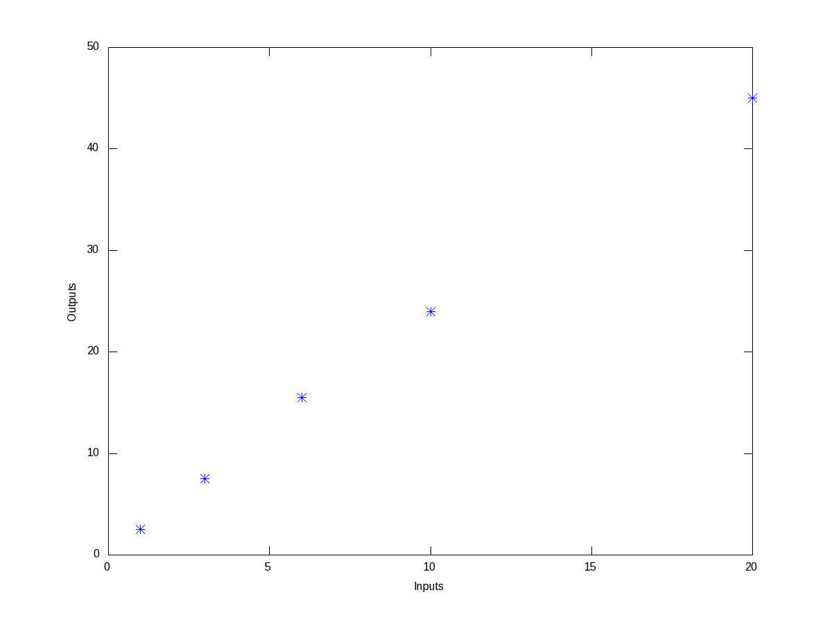
For the inputs of 1, 3, 6, 10, 20, we get the outputs as 2.5, 7.5, 15.5, 24, 45, respectively. Then, we would like to know as how is input is related to the output. So, to get a feel of the relation, we first plot this points on a x-y plane, say inputs as x and outputs as y. Figure 6 shows the same. And the octave code for that is as follows:

$ octave -qf
octave:1> x = [1 3 6 10 20];
octave:2> y = [2.5 7.5 15.5 24 45];
octave:3> plot(x, y, "*");
octave:4> xlabel("Inputs");
octave:5> ylabel("Outputs");
octave:6>
Figure 6: Plot of the data points

Figure 6: Plot of the data points

By observing the plot, the simplest fitting relation looks to be a straight line. So, let’s try fitting a linear polynomial, i.e. a first order polynomial, i.e. a straight line. Here’s the code in execution for it:

octave:1> x = [1 3 6 10 20];
octave:2> y = [2.5 7.5 15.5 24 45];
octave:3> p = polyfit(x, y, 1)
p =

   2.2212   1.1301

octave:4> polyout(p, "x");

2.2212*x^1 + 1.1301

octave:5> plot(x, y, "*", x, polyval(p, x), "-");
octave:6> xlabel("Inputs");
octave:7> ylabel("Outputs");
octave:8> legend("Data points", "Linear Fit");
octave:9>

polyfit() takes 3 arguments, the x values, the y values, and the order of the polynomial to fit – 1 for linear. It then returns the coefficients of the fitted polynomial p. polyout() displays the polynomial in more readable format. So, the fitted equation is y = 2.2212 * x + 1.1301. polyval() takes the polynomial p and the input values x, and calculates the output values y, as per the polynomial equation. And then we plot them, along with the earlier data points, on the same plot. Figure 7 shows the same, 2.2212 being the slope / gradient of the straight line, and 1.1301 being the intercept. Now, we notice that the straight line does not fit exactly, and there is some deviation from the observed points. polyfit() fits the polynomial with the minimum deviation for the order we request, but still there is a deviation, as that is the minimum possible. If you want to get the standard deviation for the particular fit, you just need to do the following:

octave:9> std_dev = sqrt(mean((y - polyval(p, x)).^2))
std_dev =  0.72637
octave:10>
Figure 7: Linear fit of data points

Figure 7: Linear fit of data points

And we see that it is a small value compared to our output values. But say we are not fully satisfied with this, we may like to try higher order polynomials, say of order 2, a quadratic, and observe the results from it. Here’s how one would do this:

octave:1> x = [1 3 6 10 20];
octave:2> y = [2.5 7.5 15.5 24 45];
octave:3> p = polyfit(x, y, 2)
p =

  -0.018639   2.623382  -0.051663

octave:4> polyout(p, "x");

-0.018639*x^2 + 2.6234*x^1 - 0.051663

octave:5> plot(x, y, "*", x, polyval(p, x), "-");
octave:6> xlabel("Inputs");
octave:7> ylabel("Outputs");
octave:8> legend("Data points", "Quadratic Fit");
octave:9> std_dev = sqrt(mean((y - polyval(p, x)).^2))
std_dev =  0.26873
octave:10>

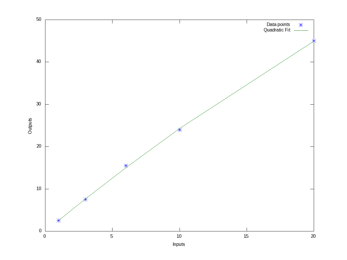
Figure 8 shows the data points and fitted quadratic curve. All the values above can be interpreted in the similar way as earlier. And we note that the standard deviation has come down further. In fact, as we increase the polynomial order further and further, we will definitely note that the standard deviation keeps on decreasing, till the order is same as number of data points – 1, after which it remains 0. But, we may not like to do this, as our observed data points are typically not perfect, and we are typically not interested in getting the standard deviation zero but for a fit more appropriate to reflect the relation between the system’s input and output.

Figure 8: Quadratic fit of data points

Figure 8: Quadratic fit of data points

Interpolation

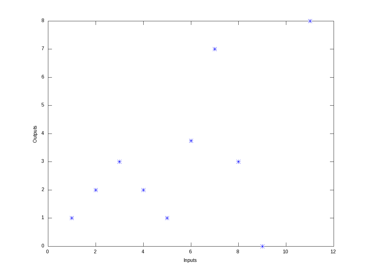
Now, say we have the following wierd data points, listed as (x, y) pairs: (1, 1), (2, 2), (3, 3), (4, 2), (5, 1), (6, 3.75), (7, 7), (8, 3), (9, 0), (11, 8). Figure 9 shows, how wierd they look like.

Figure 9: Wierd data points

Figure 9: Wierd data points

Trying to fit a polynomial, would be quite meaningless. But still they seem to have some correlation in between smaller ranges of input, say between 1 and 3, 3 and 5, 5 and 7, and so on. So, this is best suited for us to do interpolation for finding the values in between, say at 1.5, 3.8, 10, … Now interpolation is all about curve fitting between two neighbouring data points and then calculating the value at any intermediate point. So, the typical varieties of techniques used for this “piece-wise curve fitting” are:

  • nearest: Return the nearest data point (actually no curve fitting)
  • linear: Linear/Straight line fitting between the two neighbouring data points
  • pchip: Piece-wise cubic (order 3) hermite polynomial fitting
  • cubic: Cubic (order 3) polynomial fitted between four nearest neighbouring data points
  • spline: Cubic (order 3) spline fitting with smooth first and second derivatives throughout the curve

All these may look little jargonish – so don’t worry about that. Let’s just try out some examples to drive the point home. Here’s the code to show the nearest & linear interpolation for the above data:

octave:1> x = [1 2 3 4 5 6 7 8 9 11];
octave:2> y = [1 2 3 2 1 3.75 7 3 0 8];
octave:3> xi = 1:0.1:11;
octave:4> y_n = interp1(x, y, xi, "nearest");
octave:5> y_l = interp1(x, y, xi, "linear");
octave:6> plot(x, y, "*", xi, y_n, "-", xi, y_l, "-");
octave:7> xlabel("Inputs");
octave:8> ylabel("Outputs");
octave:9> legend("Data points", "Nearest", "Linear");
octave:10>

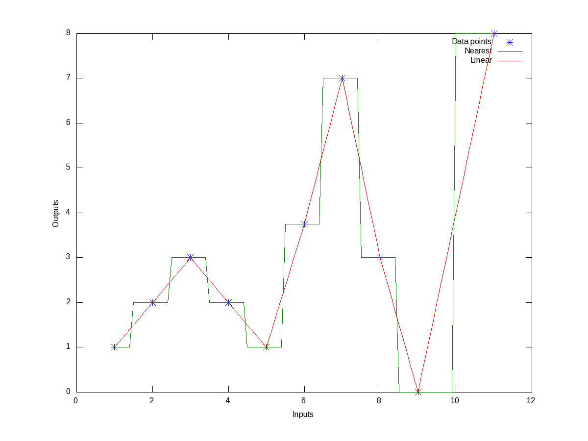
Figure 10 shows the same.

Figure 10: Nearest and linear interpolations of the data points

Figure 10: Nearest and linear interpolations of the data points

Now, if we want to get the interpolated values say at the points 1.5, 3.8, 10, instead of giving all the intermediate points xi in the above code, we may just give these 3 – that’s all. Here goes the code in execution for the that:

octave:1> x = [1 2 3 4 5 6 7 8 9 11];
octave:2> y = [1 2 3 2 1 3.75 7 3 0 8];
octave:3> our_x = [1.5 3.8 10];
octave:4> our_y_n = interp1(x, y, our_x, "nearest")
our_y_n =

   2   2   8

octave:5> our_y_l = interp1(x, y, our_x, "linear")
our_y_l =

   1.5000   2.2000   4.0000

octave:6>

Now, before closing on interpolation, just to give a feel of all of the interpolation techniques, here goes an example with the points on a sine curve:

octave:1> x = 0:2*pi;
octave:2> y = sin(x);
octave:3> xi = 0:0.1:2*pi;
octave:4> y_n = interp1(x, y, xi, "nearest");
octave:5> y_l = interp1(x, y, xi, "linear");
octave:6> y_p = interp1(x, y, xi, "pchip");
octave:7> y_c = interp1(x, y, xi, "cubic");
octave:8> y_s = interp1(x, y, xi, "spline");
octave:9> plot(x, y, "*", xi, y_n, "-", xi, y_l, "-", xi, y_p, "-", xi, y_c, "-",
                                                                      xi, y_s, "-");
octave:10> xlabel("x ->");
octave:11> ylabel("y ->");
octave:12> legend("Data points", "Nearest", "Linear", "Pchip", "Cubic", "Spline");
octave:13> print("-dpng", "all_types_of_interpolations.png");
octave:14>

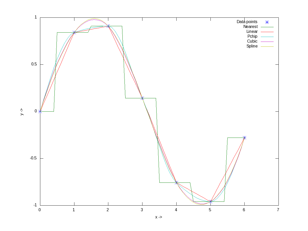
Figure 11 shows the visualization of the same for your eyes.

Figure 11: All types of interpolations for sinusoidal points

Figure 11: All types of interpolations for sinusoidal points

What’s next?

With today’s curve fitting & interpolation walk through, we have used some basic 2-D plotting techniques. But there are many more features and techniques to plotting, like marking our plots, visualizing 3-D stuff, etc. Next, we’ll look into that.

Twelfth Article >>

   Send article as PDF   

Polynomial Power of Octave

This tenth article of the mathematical journey through open source, explains advanced polynomial mathematics in octave.

<< Ninth Article

Roots of i

Let’s start with the solution to our previous brain teaser of finding the square and cube roots of the imaginary number i, which boils down to finding all the roots of the equations x2 = i and x3 = i, respectively. In other words, roots of the polynomials x2 – i and x3 – i, respectively, as follows:

$ octave -qf
octave:1> roots([1 0 -i])
ans =

   0.70711 + 0.70711i
  -0.70711 - 0.70711i

octave:2> roots([1 0 0 -i])
ans =

  -0.86603 + 0.50000i
  -0.00000 - 1.00000i
   0.86603 + 0.50000i

octave:3>

Displaying Polynomial

Before we start exploring polynomials further, here’s a couple of basic octave functions to visualize the polynomials. polyout() displays a polynomial in our usual known format. polyreduce() removes the redundant leading zero coefficients. Check out the following:

$ octave -qf
octave:1> p = [ 0 0 5 3 -9 4 6 ];
octave:2> polyout(p, "x");
0*x^6 + 0*x^5 + 5*x^4 + 3*x^3 - 9*x^2 + 4*x^1 + 6
octave:3> polyreduce(p)
ans =

   5   3  -9   4   6

octave:4> polyout(polyreduce(p), "x");
5*x^4 + 3*x^3 - 9*x^2 + 4*x^1 + 6
octave:5>

Polynomial Arithmetic

As octave represents polynomial as vectors, their addition and subtraction are vector addition and subtraction, respectively. However, the polynomial vectors may be of different length. Hence, they need to be made of same length before addition or subtraction. So, let’s write functions to do the complete operations:

function [ q1 q2 ] = equalize(p1, p2)
# Assuming p1 & p2 to be row vectors
    m = max(length(p1), length(p2));
    q1 = [ zeros(1, m - length(p1)) p1 ];
    q2 = [ zeros(1, m - length(p2)) p2 ];
endfunction

function p = polyadd(p1, p2)
    [ q1 q2 ] = equalize(p1, p2);
    p = polyreduce(q1 + q2);
endfunction

function p = polysub(p1, p2)
    [ q1 q2 ] = equalize(p1, p2);
    p = polyreduce(q1 - q2);
endfunction

Assuming the above code is put in the file polynomials.oct, the same can be used as follows:

$ octave -qf
octave:1> source("polynomials.oct");
octave:2> polyout(p1 = [ 1 2 1 ], "x");
1*x^2 + 2*x^1 + 1
octave:3> polyout(p2 = [ 1 -1 ], "x");
1*x^1 - 1
octave:4> polyout(polyadd(p1, p2), "x");
1*x^2 + 3*x^1 + 0
octave:5> polyout(polysub(p1, p2), "x");
1*x^2 + 1*x^1 + 2
octave:6>

Interestingly, octave already have the functions for multiplication and division of polynomials, namely conv() and deconv(), respectively. Here’s a demonstration:

$ octave -qf
octave:1> polyout(p1 = [ 1 2 1 ], "x");
1*x^2 + 2*x^1 + 1
octave:2> polyout(p2 = [ 1 -1 ], "x");
1*x^1 - 1
octave:3> polyout(conv(p1, p2), "x");
1*x^3 + 1*x^2 - 1*x^1 - 1
octave:4> polyout(deconv(p1, p2), "x");
1*x^1 + 3
octave:5> [ q r ] = deconv(p1, p2)
q =

   1   3

r =

   0   0   4

octave:6>

Polynomial Differentiation and Integration

Octave also provides functions for differentiation and integration of polynomials, namely polyder() and polyint(). Here goes an example of differentiation and definite integral using the same:

$ octave -qf
octave:1> polyout(p = [ 1 2 1 ], "x");
1*x^2 + 2*x^1 + 1
octave:2> polyout(polyder(p), "x");
2*x^1 + 2
octave:3> polyout(polyint(p), "x");
0.33333*x^3 + 1*x^2 + 1*x^1 + 0
octave:4> q = polyint(p);
octave:5> polyval(q, 3) - polyval(q, 0) # Definite integral of p from 0 to 3
ans =  21
octave:6>

What’s next?

Given a set of data points a common requirement in fields of physics, statistics, and many others is to fit a polynomial to it. Going further, we’ll explore the power of octave for the same.

Eleventh Article >>

   Send article as PDF   

Get Set with Polynomials in Octave

This ninth article of the mathematical journey through open source, deals with polynomial mathematics in octave.

<< Eighth Article

Let’s first solve the earlier puzzles. And then we shall discuss the polynomial power of octave.

Number Puzzle

Find three numbers, product of which is 60; sum of their squares is 50; and their sum is 12. Let the X vector elements X(1), X(2), X(3) be the three numbers. Then, here goes the solution:

$ octave -qf
octave:1> function Y = F(X)
> Y(1) = X(1) * X(2) * X(3) - 60; 
> Y(2) = X(1)^2 + X(2)^2 + X(3)^2 - 50; 
> Y(3) = X(1) + X(2) + X(3) - 12; 
> endfunction
octave:2> [Y, Fval, info] = fsolve(@F, [3; 3; 3]) 
warning: matrix singular to machine precision, rcond = 4.32582e-35
warning: attempting to find minimum norm solution
warning: dgelsd: rank deficient 3x3 matrix, rank = 1 
Y =

   5.0000
   3.0000
   4.0000

Fval =

  -3.2345e-07   1.0351e-07   0.0000e+00

info = 1 
octave:3>

So, the 3 numbers are 5, 3, 4.

Flower Puzzle

A sage came to a temple with some flowers and dipped them into the first pond of the temple to get them squared. Then, he offered some flowers in the temple and dipped the remaining flowers into the second pond to get them doubled. Then, he again offered same number of flowers, as earlier, and dipped the remaining flowers into the third pond to get them tripled and take back with him as prasadam, which was the same number as in each one of his offerings. Now, if he took back thrice the number of flowers he brought. How many did he bring in with him?
Let the x vector elements x(1) and x(2) be respectively, the number of flowers the sage came with and the number of flowers the sage offered each time. So, here goes the solution:

octave:1> function y = f(x)
> y(1) = ((x(1) * x(1) - x(2)) * 2 - x(2)) * 3 - x(2);
> y(2) = x(2) - 3 * x(1);
> endfunction 
octave:2> [x fval info] = fsolve(@f, [10; 10])
x =

    5.0000
   15.0000

fval =

  -2.8791e-06  -1.7764e-15

info =  1
octave:3>

So, the number of flowers the sage came with is 5 and his each offering is of 15 flowers.

Note that in all these solutions the trick is to choose the initial solution close to the original solution, through some approximation work. At times that might be tricky. So, in case we just have polynomial equations and that also in one variable, it can be solved in an easier way, using the polynomial features of octave. In contrast to the earlier method, here we also get all of the multiple solutions for the polynomial.

Playing with Polynomials

Let’s consider the polynomial equation 2x3 + 3x2 + 2x + 1 = 0. Then its octave representation and computation of its solutions aka roots would be as follows:

octave:1> P = [2; 3; 2; 1];
octave:2> roots(P)
ans =

  -1.00000 + 0.00000i
  -0.25000 + 0.66144i
  -0.25000 - 0.66144i

octave:3>

So, it being a cubic equation, it has three roots as expected. First one is the real number -1, and the other two are complex conjugates (-1 + sqrt(-7))/4 & (-1 – sqrt(-7))/4. And you may verify the solutions using the function polyval() as follows:

octave:1> P = [2; 3; 2; 1];
octave:2> sols = [-1; (-1 + sqrt(-7)) / 4; (-1 + sqrt(-7)) / 4]
sols =

  -1.00000 + 0.00000i
  -0.25000 + 0.66144i
  -0.25000 + 0.66144i

octave:3> polyval(P, sols)
ans =

   0
   0
   0

octave:4>

This shows that the value of the polynomial P evaluated at each of the 3 solutions is 0. Hence, confirming that they indeed are the solutions.

All set with polynomial basics in octave, let’s solve some puzzles.

Geometry Solving

Last time we found an intersection point of a straight line and a circle. Yes, we just calculated one point – though typically there would be two. It would be one only in case of the straight line being tangent or just touching the circle. And yes it would be zero, if the straight line is not even intersecting it. So now, let’s try these different cases, with the one variable polynomial power.

Let us have the following circle C with radius 5 and centered at origin (0, 0), defined in the Cartesian coordinate system, i.e. the x-y system: x2 + y2 = 25

And, let us consider the following 3 lines for intersection with the above circle, one by one:

  • L1: 4x + 3y = 24
  • L2: x + y = 5√2
  • L3: 6x + y = 36

To be able to solve for the intersection points of each of these 3 lines with the circle C using roots, the first step is to get polynomials in one variable. For that, we can substitute the value of y in the equation of the circle, in terms of x from each of the line equations, as follows:
For L1
x2 + y2 = 25 ⇒ 9x2 + 9y2 = 9*25 ⇒ 9x2 + (24 – 4x)2 = 225 ⇒ 25x2 – 192x + 351 = 0
For L2
x2 + y2 = 25 ⇒ x2 + (5√2 – x)2 = 25 ⇒ 2x2 – 10√2x + 25 = 0
For L3
x2 + y2 = 25 ⇒ x2 + (36 – 6x)2 = 25 ⇒ 37x2 – 432x + 1271 = 0

Now, we get the roots of each to get the x co-ordinate of the intersection point.

octave:1> C1 = [25; -192; 351];
octave:2> C2 = [2; -10*sqrt(2); 25];
octave:3> C3 = [37; -432; 1271];
octave:4> roots(C1)
ans =

   4.6800
   3.0000

octave:5> roots(C2)
ans =

   3.5355
   3.5355

octave:6> roots(C3)
ans =

   5.8378 + 0.5206i
   5.8378 - 0.5206i

octave:7>

And the corresponding y co-ordinate could be obtained by substituting the value of x into the corresponding line equations.

For L1, there are 2 different roots 4.68 and 3, implying two intersecting points (4.68, 1.76) and (3, 4).
For L2, there are 2 identical roots of 3.5355 i.e 5/√2, implying just one intersecting point (5/√2, 5/√2).
For L3, the roots are complex, implying that there is no intersecting point in the real world.

Solve it

And finally, here’s one for your brain. Find out the two square roots and the three cube roots of the imaginary number i.

If you think, you have got the octave code for solving the above, post your solution in the comments below. And as we move on, we would have more fun with the polynomials.

Tenth Article >>

   Send article as PDF