This twenty-fourth article of the mathematical journey through open source, demonstrates the concepts of graph theory for playing with graphs using the graphs package of Maxima.
<< Twenty-third Article
In our previous article, we familiarized ourselves with the notion of simple graphs, and how graphs package of Maxima allows us to create and visualize them. Assuming that knowledge, in this article, we are going to play with graphs and their properties, using the functionalities provided by Maxima’s graphs package.
Graph modifications
We have already created various graphs with create_graph() and make_graph() functions of the graphs package of Maxima. What if we want to modify some existing graphs, say by adding or removing some edges or vertices? Exactly for such operations, Maxima provides the following functions:
- add_edge(<edge>, <g>) – Adds <edge> into the graph <g>
- add_edges(<edge_list>, <g>) – Adds edges specified by <edge_list> into the graph <g>
- add_vertex(<vertex>, <g>) – Adds <vertex> into the graph <g>
- add_vertices(<vertex_list>, <g>) – Adds vertices specified by <vertex_list> into the graph <g>
- connect_vertices(<u_list>, <v_list>, <g>) – Connects all vertices from <u_list> to all vertices in <v_list> in the graph <g>
- contract_edge(<edge>, <g>) – Merges the vertices of the <edge> and the edges incident on those vertices, in the graph <g>
- remove_edge(<edge>, <g>) – Removes the <edge> from the graph <g>
- remove_vertex(<vertex>, <g>) – Removes the <vertex> and the associated edges from the graph <g>
Some of the above functions are demonstrated below:
$ maxima -q
(%i1) load(graphs)$ /* Loading the graphs package */
...
0 errors, 0 warnings
(%i2) g: create_graph(4, [[0, 1], [0, 2]]);
(%o2)                     GRAPH(4 vertices, 2 edges)
(%i3) print_graph(g)$

Graph on 4 vertices with 2 edges.
Adjacencies:
  3 :
  2 :  0
  1 :  0
  0 :  2  1
(%i4) add_edge([1, 2], g)$
(%i5) print_graph(g)$

Graph on 4 vertices with 3 edges.
Adjacencies:
  3 :
  2 :  1  0
  1 :  2  0
  0 :  2  1
(%i6) contract_edge([0, 1], g)$
(%i7) print_graph(g)$

Graph on 3 vertices with 1 edges.
Adjacencies:
  3 :
  2 :  0
  0 :  2
In the above examples, if we do not intend to modify the original graph, we may make a copy of it using copy_graph(), and then operate on the copy, as follows:
(%i8) h: copy_graph(g);
(%o8)                     GRAPH(3 vertices, 1 edges)
(%i9) add_vertex(1, h)$
(%i10) print_graph(h)$

Graph on 4 vertices with 1 edges.
Adjacencies:
  1 :
  0 :  2
  2 :  0
  3 :
(%i11) print_graph(g)$ /* Notice g is unmodified */

Graph on 3 vertices with 1 edges.
Adjacencies:
  3 :
  2 :  0
  0 :  2
(%i12) quit();
Advanced graph creations
New graphs can also be created based on existing graphs and their properties by various interesting operations. Few of them are:
- underlying_graph(<dg>) – Returns the underlying graph of the directed graph <dg>
- complement_graph(<g>) – Returns the complement graph of graph <g>
- line_graph(<g>) – Returns a graph that represents the adjacencies between the edges of graph <g>
- graph_union(<g1>, <g2>) – Returns a graph with edges and vertices of both graphs <g1> and <g2>
- graph_product(<g1>, <g2>) – Returns the Cartesian product of graphs <g1> and <g2>
Here are some examples to demonstrate the simpler functions:
$ maxima -q
(%i1) load(graphs)$
...
0 errors, 0 warnings
(%i2) g: create_graph(4, [[0, 1], [0, 2], [0, 3]], directed = true);
(%o2)                     DIGRAPH(4 vertices, 3 arcs)
(%i3) print_graph(g)$

Digraph on 4 vertices with 3 arcs.
Adjacencies:
  3 :
  2 :
  1 :
  0 :  3  2  1
(%i4) h: underlying_graph(g);
(%o4)                     GRAPH(4 vertices, 3 edges)
(%i5) print_graph(h)$

Graph on 4 vertices with 3 edges.
Adjacencies:
  0 :  1  2  3
  1 :  0
  2 :  0
  3 :  0
(%i6) print_graph(complement_graph(h))$

Graph on 4 vertices with 3 edges.
Adjacencies:
  3 :  2  1
  2 :  3  1
  1 :  3  2
  0 :
(%i7) print_graph(graph_union(h, complement_graph(h)))$

Graph on 8 vertices with 6 edges.
Adjacencies:
  4 :
  5 :  6  7
  6 :  5  7
  7 :  5  6
  3 :  0
  2 :  0
  1 :  0
  0 :  3  2  1
(%i8) quit();
Basic graph properties
graph_order(<g>), vertices(<g>) returns the number of vertices and the list of vertices, respectively, in the graph <g>. graph_size(<g>), edges(<g>) returns the number of edges and the list of edges, respectively, in the graph <g>.
A graph is a collection of vertices and edges. Hence, most of its properties are centred around them. The following are graph related predicates provided by the graphs package of Maxima:
- is_graph(<g>) – returns true if <g> is a graph, false otherwise
- is_digraph(<g>) – returns true if <g> is a directed graph, false otherwise
- is_graph_or_digraph(<g>) – returns true if <g> is a graph or a directed graph, false otherwise
- is_connected(<g>) – returns true if graph <g> is connected, false otherwise
- is_planar(<g>) – returns true if graph <g> can be placed on a plane without its edges crossing over each other, false otherwise
- is_tree(<g>) – returns true if graph <g> has no simple cycles, false otherwise
- is_biconnected(<g>) – returns true if graph <g> will remain connected even after removal of any one its vertices and the edges incident on that vertex, false otherwise
- is_bipartite(<g>) – returns true if graph <g> is bipartite, i.e. 2-colourable, false otherwise
- is_isomorphic(<g1>, <g2>) – returns true if graphs <g1> and <g2> have the same number of vertices and are connected in the same way, false otherwise. And, isomorphism(<g1>, <g2>) returns an isomorphism (that is a one-to-one onto mapping) between the graphs <g1> and <g2>, if it exists.
- is_edge_in_graph(<edge>, <g>) – returns true if <edge> is in graph <g>, false otherwise
- is_vertex_in_graph(<vertex>, <g>) – returns true if <vertex> is in graph <g>, false otherwise
The following example specifically demonstrates the isomorphism property, from the list above:
$ maxima -q
(%i1) load(graphs)$
...
0 errors, 0 warnings
(%i2) g1: create_graph(3, [[0, 1], [0, 2]]);
(%o2)                     GRAPH(3 vertices, 2 edges)
(%i3) g2: create_graph(3, [[1, 2], [0, 2]]);
(%o3)                     GRAPH(3 vertices, 2 edges)
(%i4) is_isomorphic(g1, g2);
(%o4)                                true
(%i5) isomorphism(g1, g2);
(%o5)                      [2 -> 0, 1 -> 1, 0 -> 2]
(%i6) quit();
Graph neighbourhoods
Lot of properties of graphs are to do with vertex and edge neighbourhoods, also referred as adjacencies.
For example, a graph itself could be represented by an adjacency list or matrix, which specifies the vertices adjacent to the various vertices in the graph. adjacency_matrix(<g>) returns the adjacency matrix of the graph <g>.
Number of edges incident on a vertex is called the valency or degree of the vertex, and could be obtained using vertex_degree(<v>, <g>). degree_sequence(<g>) returns the list of degrees of all the vertices of the graph <g>. In case of a directed graph, the degrees could be segregated as in-degree and out-degree, as per the edges incident into and out of the vertex, respectively. vertex_in_degree(<v>, <dg>) and vertex_out_degree(<v>, <dg>) respectively return the in-degree and out-degree for the vertex <v> of the directed graph <dg>.
neighbors(<v>, <g>), in_neighbors(<v>, <dg>), out_neighbors(<v>, <dg>) respectively return the list of adjacent vertices, adjacent in-vertices, adjacent out-vertices of the vertex <v> in the corresponding graphs.
average_degree(<g>) computes the average of degrees of all the vertices of the graph <g>. max_degree(<g>) finds the maximal degree of vertices of the graph <g>, and returns one such vertex alongwith. min_degree(<g>) finds the minimal degree of vertices of the graph <g>, and returns one such vertex alongwith.
Here follows a neighbourhood related demonstration:
$ maxima -q
(%i1) load(graphs)$
...
0 errors, 0 warnings
(%i2) g: create_graph(4, [[0, 1], [0, 2], [0, 3], [1, 2]]);
(%o2)                     GRAPH(4 vertices, 4 edges)
(%i3) string(adjacency_matrix(g)); /* string for output in single line */
(%o3)           matrix([0,0,0,1],[0,0,1,1],[0,1,0,1],[1,1,1,0])
(%i4) degree_sequence(g);
(%o4)                            [1, 2, 2, 3]
(%i5) average_degree(g);
(%o5)                                  2
(%i6) neighbors(0, g);
(%o6)                              [3, 2, 1]
(%i7) quit();
Graph connectivity
A graph is ultimately about connections, and hence lots of graph properties are centred around connectivity.
vertex_connectivity(<g>) returns the minimum number of vertices that need to be removed from the graph <g> to make the graph <g> disconnected. Similarly, edge_connectivity(<g>) returns the minimum number of edges that need to be removed from the graph <g> to make the graph <g> disconnected.
vertex_distance(<u>, <v>, <g>) returns the length of the shortest path between the vertices <u> and <v> in the graph <g>. The actual path could be obtained using shortest_path(<u>, <v>, <g>).
girth(<g>) returns the length of the shortest cycle in graph <g>.
vertex_eccentricity(<v>, <g>) returns the maximum of the vertex distances of vertex <v> with any other vertex in the connected graph <g>.
diameter(<g>) returns the maximum of the vertex eccentricities of all the vertices in the connected graph <g>.
radius(<g>) returns the minimum of the vertex eccentricities of all the vertices in the connected graph <g>.
graph_center(<g>) returns the list of vertices that have eccentricities equal to the radius of the connected graph <g>.
graph_periphery(<g>) is the list of vertices that have eccentricities equal to the diameter of the connected graph.
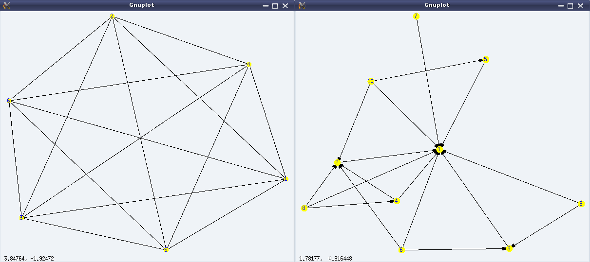
A minimal connectivity related demonstration for the graph shown in Figure 29 follows:
$ maxima -q
(%i1) load(graphs)$
...
0 errors, 0 warnings
(%i2) g: create_graph(9, [[0, 1], [0, 2], [1, 8], [8, 3], [2, 3], [3, 4], [4, 5],
        [3, 6], [3, 7]]);
(%o2)                     GRAPH(9 vertices, 9 edges)
(%i3) vertex_connectivity(g);
(%o3)                                  1
(%i4) edge_connectivity(g);
(%o4)                                 1
(%i5) shortest_path(0, 7, g);
(%o5)                           [0, 2, 3, 7]
(%i6) vertex_distance(0, 7, g);
(%o6)                                 3
(%i7) girth(g);
(%o7)                                 5
(%i8) diameter(g);
(%o8)                                 4
(%i9) radius(g);
(%o9)                                 2
(%i10) graph_center(g);
(%o10)                                [3]
(%i11) graph_periphery(g);
(%o11)                             [5, 1, 0]
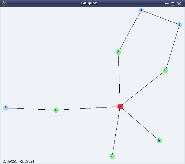
Figure 29: Graph connectivities
Vertex 3 is the only centre of the graph and 0, 1, 5 are the peripheral vertices of the graph.
Graph colouring
Graph colouring has been a fascinating topic in graph theory, since its inception. It is all about colouring the vertices or edges of a graph in such a way that no adjacent elements (vertex or edge) have the same colour.
Smallest number of colours needed to colour the vertices of a graph, such that no two adjacent vertices have the same colour, is called the chromatic number of the graph. chromatic_number(<g>) computes the same. vertex_coloring(<g>) returns a list representing the colouring of the vertices of <g>, along with the chromatic number.
Smallest number of colours needed to colour the edges of a graph, such that no two adjacent edges have the same colour, is called the chromatic index of the graph. chromatic_index(<g>) computes the same. edge_coloring(<g>) returns a list representing the colouring of the edges of <g>, along with the chromatic index.
The following demonstration continues colouring the graph from the above demonstration:
(%i12) chromatic_number(g);
(%o12)                                 3
(%i13) vc: vertex_coloring(g);
(%o13) [3, [[0, 3], [1, 1], [2, 2], [3, 1], [4, 2], [5, 1], [6, 2], [7, 2], [8, 2]]]
(%i14) chromatic_index(g);
(%o14)                                 5
(%i15) ec: edge_coloring(g);
(%o15) [5, [[[0, 1], 1], [[0, 2], 2], [[1, 8], 2], [[3, 8], 5], [[2, 3], 1],
                           [[3, 4], 2], [[4, 5], 1], [[3, 6], 3], [[3, 7], 4]]]
(%i16) draw_graph(g, vertex_coloring=vc, edge_coloring=ec, vertex_size=5,
        edge_width=3, show_id=true)$
(%i17) quit();
Figure 30 shows the coloured version of the graph, as obtained by %i16.
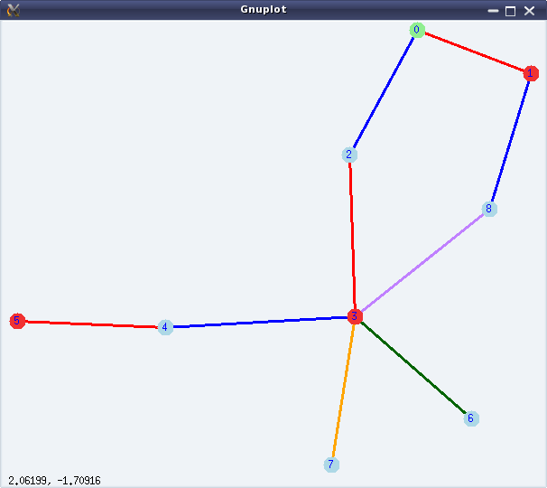
Figure 30: Graph colouring
Bon voyage
With this article, we have completed a 2 year long mathematical journey through open source, starting from mathematics in Shell, covering Bench Calculator, Octave, and finally concluding with Maxima. I take this opportunity to thank my readers and wish them bon voyage with whatever they have gained through our interactions. However, this is not the end – get set for our next odyssey.