Tag Archives: LFY

Understanding the Partitions: A dive inside the hard disk

This fourteenth article, which is part of the series on Linux device drivers, takes you for a walk inside a hard disk.

<< Thirteenth Article

Hard disk design

“Doesn’t it sound like a mechanical engineering subject: Design of hard disk?”, questioned Shweta. “Yes, it does. But understanding it gets us an insight into its programming aspect”, reasoned Pugs while waiting for the commencement of the seminar on storage systems.

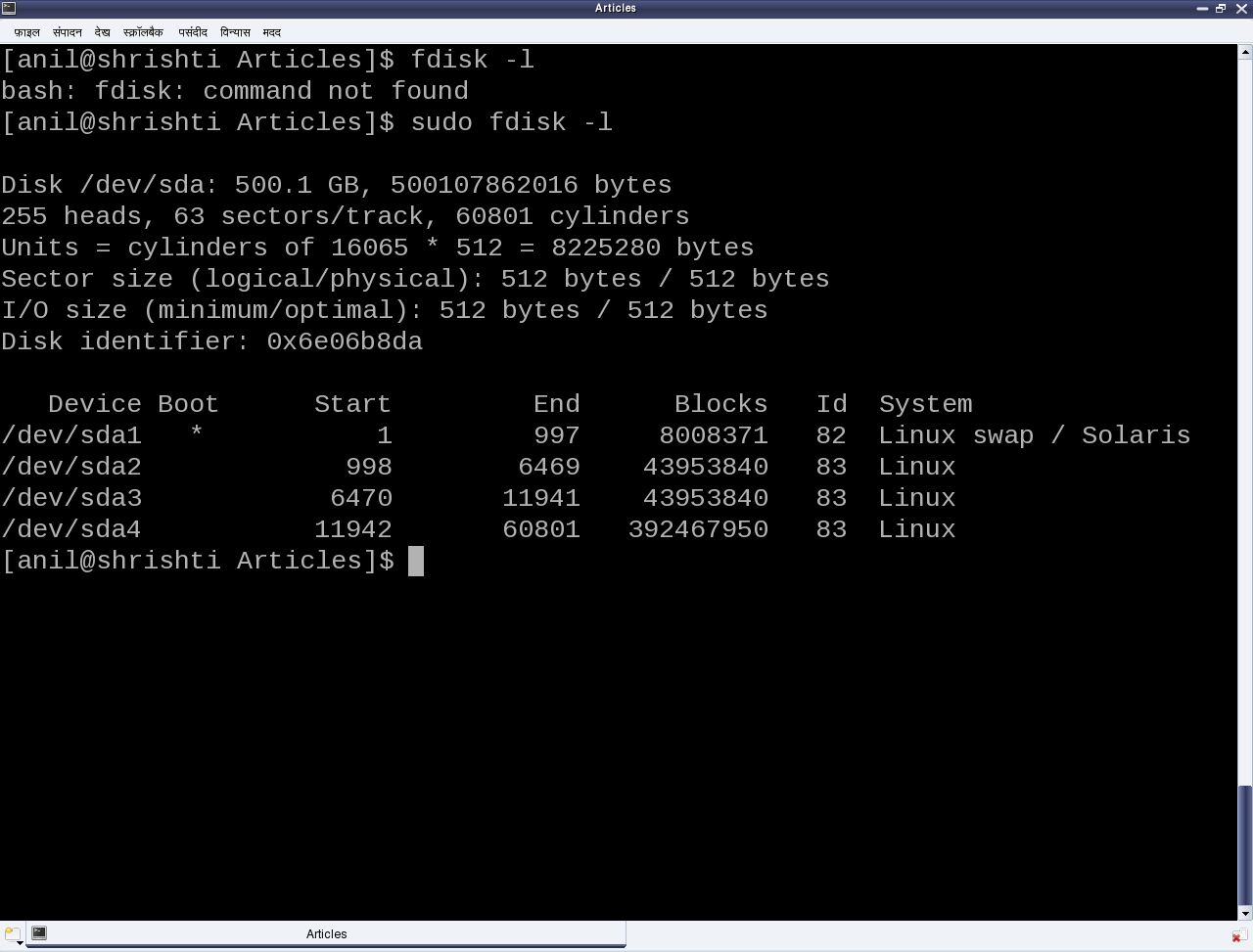
Figure 23: Partition listing by fdisk

Figure 23: Partition listing by fdisk

The seminar started with a few hard disks in the presenter’s hand and then a dive down into her system showing the output of fdisk -l, as shown in Figure 23. The first line shows the hard disk size in human friendly format and in bytes. The second line mentions the number of logical heads, logical sectors per track, and the actual number of cylinders on the disk – these together are referred as the geometry of the disk. The 255 heads indicating the number of platters or disks, as one read-write head is needed per disk. Let’s number them say D1, D2, …, D255. Now, each disk would have the same number of concentric circular tracks, starting from outside to inside. In the above case there are 60801 such tracks per disk. Let’s number them say T1, T2, …, T60801. And a particular track number from all the disks forms a cylinder of the same number. For example, tracks T2 from D1, D2, …, D255 will all together form the cylinder C2. Now, each track has the same number of logical sectors – 63 in our case, say S1, S2, …, S63. And each sector is typically 512 bytes. Given this data, one can actually compute the total usable hard disk size, using the following formula:

Usable hard disk size in bytes = (Number of heads or disks) * (Number of tracks per disk) * (Number of sectors per track) * (Number of bytes per sector, i.e. sector size).

For the disk under consideration it would be: 255 * 60801 * 63 * 512 bytes = 500105249280 bytes. Note that this number may be slightly less than the actual hard disk – 500107862016 bytes in our case. The reason for that is that the formula doesn’t consider the bytes in last partial or incomplete cylinder. And the primary reason for that is the difference between today’s technology of organizing the actual physical disk geometry and the traditional geometry representation using heads, cylinders, sectors. Note that in the fdisk output, we referred to the heads, and sectors per track as logical not the actual one. One may ask, if today’s disks doesn’t have such physical geometry concepts, then why to still maintain that and represent them in more of logical form. The main reason is to be able to continue with same concepts of partitioning and be able to maintain the same partition table formats especially for the most prevalent DOS type partition tables, which heavily depend on this simplistic geometry. Note the computation of cylinder size (255 heads * 63 sectors / track * 512 bytes / sector = 8225280 bytes) in the third line and then the demarcation of partitions in units of complete cylinders.

DOS type partition tables

This brings us to the next important topic of understanding the DOS type partition tables. But in the first place, what is a partition and rather why to even partition? A hard disk can be divided into one more logical disks, each of which is called a partition. And this is useful for organizing different types of data separately. For example, different operating system data, user data, temporary data, etc. So, partitions are basically logical divisions and hence need to be maintained through some meta data, which is the partition table. A DOS type partition table contains 4 partition entries, each being a 16-byte entry. And each of these entries can be depicted by the following ‘C’ structure:

typedef struct
{
	unsigned char boot_type; // 0x00 - Inactive; 0x80 - Active (Bootable)
	unsigned char start_head;
	unsigned char start_sec:6;
	unsigned char start_cyl_hi:2;
	unsigned char start_cyl;
	unsigned char part_type;
	unsigned char end_head;
	unsigned char end_sec:6;
	unsigned char end_cyl_hi:2;
	unsigned char end_cyl;
	unsigned int abs_start_sec;
	unsigned int sec_in_part;
} PartEntry;

And this partition table followed by the two-byte signature 0xAA55 resides at the end of hard disk’s first sector, commonly known as Master Boot Record or MBR (in short). Hence, the starting offset of this partition table within the MBR is 512 – (4 * 16 + 2) = 446. Also, a 4-byte disk signature is placed at the offset 440. The remaining top 440 bytes of the MBR are typically used to place the first piece of boot code, that is loaded by the BIOS to boot up the system from the disk. Listing of part_info.c contains these various defines, and the code for parsing and printing a formatted output of the partition table of one’s hard disk.

From the partition table entry structure, it could be noted that the start and end cylinder fields are only 10 bits long, thus allowing a maximum of 1023 cylinders only. However, for today’s huge hard disks, this size is no way sufficient. And hence in overflow cases, the corresponding <head, cylinder, sector> triplet in the partition table entry is set to the maximum value, and the actual value is computed using the last two fields: the absolute start sector number (abs_start_sec) and the number of sectors in this partition (sec_in_part). Listing of part_info.c contains the code for this as well.

#include <stdio.h>
#include <sys/types.h>
#include <sys/stat.h>
#include <fcntl.h>
#include <unistd.h>

#define MBR_DISK_SIGNATURE_OFFSET 440
#define PARTITION_ENTRY_SIZE 16 // sizeof(PartEntry)
#define PARTITION_TABLE_SIZE (4 * PARTITION_ENTRY_SIZE)

typedef struct
{
	unsigned char boot_type; // 0x00 - Inactive; 0x80 - Active (Bootable)
	unsigned char start_head;
	unsigned char start_sec:6;
	unsigned char start_cyl_hi:2;
	unsigned char start_cyl;
	unsigned char part_type;
	unsigned char end_head;
	unsigned char end_sec:6;
	unsigned char end_cyl_hi:2;
	unsigned char end_cyl;
	unsigned int abs_start_sec;
	unsigned int sec_in_part;
} PartEntry;

typedef struct
{
	unsigned char boot_code[MBR_DISK_SIGNATURE_OFFSET];
	unsigned int disk_signature;
	unsigned short pad;
	unsigned char pt[PARTITION_TABLE_SIZE];
	unsigned short signature;
} MBR;

void print_computed(unsigned int sector)
{
	unsigned int heads, cyls, tracks, sectors;

	sectors = sector % 63 + 1 /* As indexed from 1 */;
	tracks = sector / 63;
	cyls = tracks / 255 + 1 /* As indexed from 1 */;
	heads = tracks % 255;
	printf("(%3d/%5d/%1d)", heads, cyls, sectors);
}

int main(int argc, char *argv[])
{
	char *dev_file = "/dev/sda";
	int fd, i, rd_val;
	MBR m;
	PartEntry *p = (PartEntry *)(m.pt);

	if (argc == 2)
	{
		dev_file = argv[1];
	}
	if ((fd = open(dev_file, O_RDONLY)) == -1)
	{
		fprintf(stderr, "Failed opening %s: ", dev_file);
		perror("");
		return 1;
	}
	if ((rd_val = read(fd, &m, sizeof(m))) != sizeof(m))
	{
		fprintf(stderr, "Failed reading %s: ", dev_file);
		perror("");
		close(fd);
		return 2;
	}
	close(fd);
	printf("\nDOS type Partition Table of %s:\n", dev_file);
	printf("  B Start (H/C/S)   End (H/C/S) Type  StartSec    TotSec\n");
	for (i = 0; i < 4; i++)
	{
		printf("%d:%d (%3d/%4d/%2d) (%3d/%4d/%2d)  %02X %10d %9d\n",
			i + 1, !!(p[i].boot_type & 0x80),
			p[i].start_head,
			1 + ((p[i].start_cyl_hi << 8) | p[i].start_cyl),
			p[i].start_sec,
			p[i].end_head,
			1 + ((p[i].end_cyl_hi << 8) | p[i].end_cyl),
			p[i].end_sec,
			p[i].part_type,
			p[i].abs_start_sec, p[i].sec_in_part);
	}
	printf("\nRe-computed Partition Table of %s:\n", dev_file);
	printf("  B Start (H/C/S)   End (H/C/S) Type  StartSec    TotSec\n");
	for (i = 0; i < 4; i++)
	{
		printf("%d:%d ", i + 1, !!(p[i].boot_type & 0x80));
		print_computed(p[i].abs_start_sec);
		printf(" ");
		print_computed(p[i].abs_start_sec + p[i].sec_in_part - 1);
		printf(" %02X %10d %9d\n", p[i].part_type,
			p[i].abs_start_sec, p[i].sec_in_part);
	}
	printf("\n");
	return 0;
}

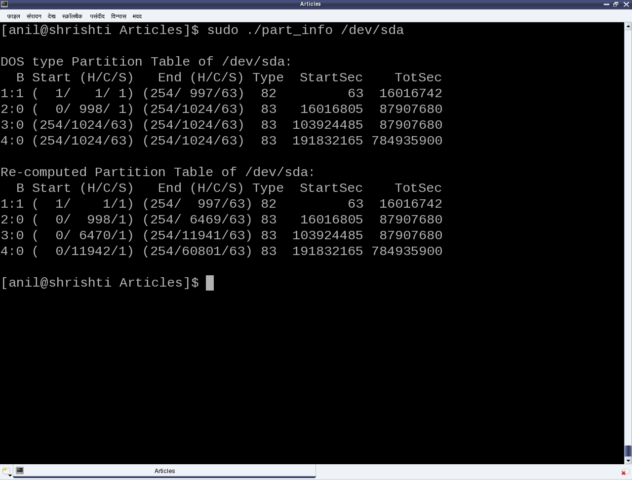
As the above code (part_info.c) is an application, compile it to an executable (./part_info) as follows: gcc part_info.c -o part_info, and then run ./part_info /dev/sda to check out your primary partitioning information on /dev/sda. Figure 24 shows the output of ./part_info on the presenter’s system. Compare it with the fdisk output as shown in figure 23.

Figure 24: Output of ./part_info

Figure 24: Output of ./part_info

Partition types and Boot records

Now as this partition table is hard-coded to have 4 entries, that dictates the maximum number of partitions, we can have, namely 4. These are called primary partitions, each having a type associated with them in their corresponding partition table entry. The various types are typically coined by the various operating system vendors and hence it is a sort of mapping to the various operating systems, for example, DOS, Minix, Linux, Solaris, BSD, FreeBSD, QNX, W95, Novell Netware, etc to be used for/with the particular operating system. However, this is more of ego and formality than a real requirement.

Apart from these, one of the 4 primary partitions can actually be labeled as something referred as an extended partition, and that has a special significance. As name suggests, it is used to further extend the hard disk division, i.e. to have more partitions. These more partitions are referred as logical partitions and are created within the extended partition. Meta data of the logical partitions is maintained in a linked list format, allowing unlimited number of logical partitions, at least theoretically. For that, the first sector of the extended partition, commonly referred to as Boot Record or BR (in short), is used in a similar way as MBR to store (the linked list head of) the partition table for the logical partitions. Subsequent linked list nodes are stored in the first sector of the subsequent logical partitions, referred to as Logical Boot Record or LBR (in short). Each linked list node is a complete 4-entry partition table, though only the first two entries are used – the first for the linked list data, namely, information about the immediate logical partition, and second one as the linked list’s next pointer, pointing to the list of remaining logical partitions.

To compare and understand the primary partitioning details on your system’s hard disk, follow these steps (as root user and hence with care):

  • ./part_info /dev/sda # Displays the partition table on /dev/sda
  • fdisk -l /dev/sda # To display and compare the partition table entries with the above

In case you have multiple hard disks (/dev/sdb, …), or hard disk device file with other names (/dev/hda, …), or an extended partition, you may try ./part_info <device_file_name> on them as well. Trying on an extended partition would give the information about the starting partition table of the logical partitions.

Summing up

“Right now we carefully and selectively played (read only) with our system’s hard disk. Why carefully? As otherwise, we may render our system non-bootable. But no learning is complete without a total exploration. Hence, in our post-lunch session, we would create a dummy disk on RAM and do the destructive explorations.”
Fifteenth Article >>

   Send article as PDF   

Doing Algebra with Maxima

This fourteenth article of the mathematical journey through open source, introduces to doing algebra using Maxima.

<< Thirteenth Article

Maxima is a computer algebra system derived from the earlier Macsyma, which in turn, was written in Lisp.

Algebraic capability of Maxima is the one, which puts it apart from the others. We have worked through basic shell maths, bench calculator bc, and finally the ultra capable octave. But none of them could do algebra with symbols, also referred as symbolic or analytic mathematics. Let’s walk through a few examples to demonstrate what it means.

Getting started

Maxima command line can be started on the shell by typing maxima. -q option to it suppresses the initial welcome message. Typing quit(); on the Maxima command line quits Maxima. Typical Maxima commands shall be terminated either with a semicolon (;) or a dollar ($) – the later suppressing any print from the command. Outputs are numbered and prefaced by %o. Inputs are also numbered, and prefaced by %i. Here are a few factorization examples:

$ maxima -q
(%i1) factor(x^3 - 1);
                                       2
(%o1)                        (x - 1) (x  + x + 1)
(%i2) factor((x + 1)^4);
                                     4
(%o2)                              (x + 1)
(%i3) expand(%o2);
                           4      3      2
(%o3)                     x  + 4 x  + 6 x  + 4 x + 1
(%i4) factor(6!);
                                     4  2
(%o4)                               2  3  5
(%i5) expand(6!);
(%o5)                                 720
(%i6) quit();

factor() and expand() are two complementary functions doing factorization & simplification, respectively. Note the way the powers in the output are printed. For example, 6! is factorized as 24 * 32 * 5. In case, we want the output on a single line, we may use the command string(), which we shall use now onwards. Also, note the usage of output labels as inputs to the commands, namely expand(%o2) in the above example.

Integration and differentiation

Octave has enabled us to do integration and differentiation, but more of definite integrals and differences. Yes, it has indefinite operations for polynomials. But with Maxima, we can just plug in the expressions, as we usually do on our maths notebooks. This is what it means:

$ maxima -q
(%i1) integrate(cos(x),x);
(%o1)                               sin(x)
(%i2) diff(cos(x),x);
(%o2)                              - sin(x)
(%i3) string(integrate(1/(a^2 + x^2)^(3/2),x));
(%o3)                        x/(a^2*sqrt(x^2+a^2))
(%i4) string(diff(log(x), x));
(%o4)                                 1/x
(%i5) y: (x+1)^2$ /* $ suppresses the output */
(%i6) string(diff(y, x));
(%o6)                              2*(x+1)
(%i7) string(integrate(y, x));
(%o7)                            x^3/3+x^2+x
(%i8) quit();

Variable assignments can be done in Maxima using colon (:), as shown in the input %i5, above. There onwards, the variable can be used instead of the original expression, as shown in the inputs %i6 & %i7. Note that the variable assignment assigns the complete symbolic expression, unlike the usual value assignments.

Solving equations

Whether it be linear set of equations, polynomial equations, or for that matter non-linear equations, Maxima can solve most of them with quite ease, and that also in a analytical way. Here are a few common examples: 1) The two solutions of a quadratic equation; 2) Two simultaneous equations in two variables; 3) A non-linear equation with irrational number e. Maxima code demonstration follows:

$ maxima -q
(%i1) string(solve(a*x^2 + b*x + c = 0, x));
(%o1)   [x = -(sqrt(b^2-4*a*c)+b)/(2*a),x = (sqrt(b^2-4*a*c)-b)/(2*a)]
(%i2) string(solve([a*x + b*y = c,d*x + e*y = f],[x, y]));
(%o2)        [[x = -(c*e-b*f)/(b*d-a*e),y = (c*d-a*f)/(b*d-a*e)]]
(%i3) string(solve([exp(x) + 1/exp(x) = a],[x]));
(%o3)      [x = log(a/2-sqrt(a^2-4)/2),x = log(sqrt(a^2-4)/2+a/2)]
(%i8) quit();

Equation solving has been one of the most fascinating as well as challenging tasks for solving mathematical problems, since ages. So, when the computer is there to aid it, we try to go beyond the human limitations. We just saw the well-known formula for the two solutions of a quadratic equation. How about the same for a cubic equation? It looks really complicated and hence we typically don’t use it. But, still you want to see it. Here it goes:

$ maxima -q
(%i1) string(solve(a*x^3 + b*x^2 + c*x + d = 0, x));
(%o1) [x = (-sqrt(3)*%i/2-1/2)*(sqrt(27*a^2*d^2+(4*b^3-18*a*b*c)*d+4*a*c^3-b^2*c^2)/
(2*3^(3/2)*a^2)-(27*a^2*d-9*a*b*c+2*b^3)/(54*a^3))^(1/3)-(sqrt(3)*%i/2-1/2)*(3*a*c-
b^2)/(9*a^2*(sqrt(27*a^2*d^2+(4*b^3-18*a*b*c)*d+4*a*c^3-b^2*c^2)/(2*3^(3/2)*a^2)-
(27*a^2*d-9*a*b*c+2*b^3)/(54*a^3))^(1/3))-b/(3*a),x = (sqrt(3)*%i/2-1/2)*(sqrt(27*
a^2*d^2+(4*b^3-18*a*b*c)*d+4*a*c^3-b^2*c^2)/(2*3^(3/2)*a^2)-(27*a^2*d-9*a*b*c+2*b^3)/
(54*a^3))^(1/3)-(-sqrt(3)*%i/2-1/2)*(3*a*c-b^2)/(9*a^2*(sqrt(27*a^2*d^2+(4*b^3-18*a*
b*c)*d+4*a*c^3-b^2*c^2)/(2*3^(3/2)*a^2)-(27*a^2*d-9*a*b*c+2*b^3)/(54*a^3))^(1/3))-b/
(3*a),x = (sqrt(27*a^2*d^2+(4*b^3-18*a*b*c)*d+4*a*c^3-b^2*c^2)/(2*3^(3/2)*a^2)-(27*
a^2*d-9*a*b*c+2*b^3)/(54*a^3))^(1/3)-(3*a*c-b^2)/(9*a^2*(sqrt(27*a^2*d^2+(4*b^3-18*
a*b*c)*d+4*a*c^3-b^2*c^2)/(2*3^(3/2)*a^2)-(27*a^2*d-9*a*b*c+2*b^3)/(54*a^3))^(1/3))-
b/(3*a)]
(%i2) quit();

And that’s what is the power of Maxima.

Plotting graphs

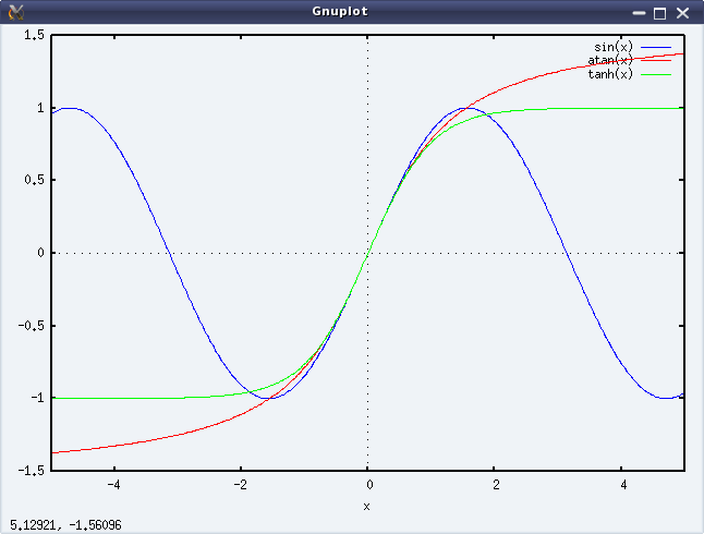
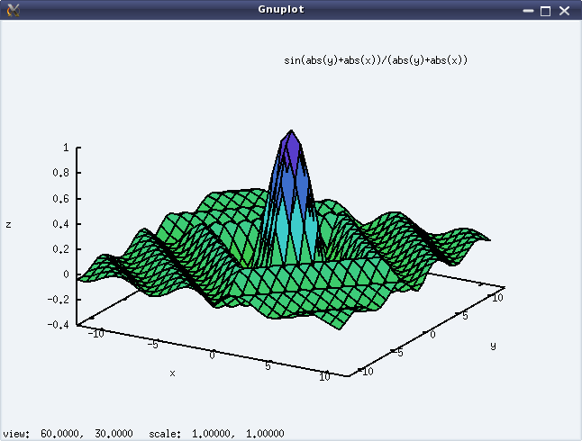
Along with the algebraic processing, Maxima also supports graph plotting for the algebraic expressions, though we must specify the intervals to plot it. It can do 2-D as well as 3-D plots. The following code shows an example for each of these. And figures 22 & 23 show the respective plots.

$ maxima -q
(%i1) plot2d([sin(x), atan(x), tanh(x)], [x, -5, 5])$
(%i2) plot3d(sin(abs(x) + abs(y))/(abs(x) + abs(y)),[x, -12, 12], [y, -12, 12])$
(%i3) quit();
Figure 22: Output of plot2d()

Figure 22: Output of plot2d()

Figure 23: Output of plot3d()

Figure 23: Output of plot3d()

After this first glimpse of what Maxima can do, we are now ready to move on to detail out the specific topics, like expression simplification, polynomials, etc.

Fifteenth Article >>

   Send article as PDF   

USB Drivers in Linux: Data Transfer to & from USB Devices

This thirteenth article, which is part of the series on Linux device drivers, details out the ultimate step of data transfer to and from a USB device using your first USB driver in Linux – a continuation from the previous two articles.

<< Twelfth Article

USB miscellany

Pugs continued, “To answer your question about how a driver selectively registers or skips a particular interface of a USB device, you need to understand the significance of the return value of probe() callback.” Note that the USB core would invoke probe for all the interfaces of a detected device, except the ones which are already registered. So, for the first time, it would call for all. Now, if the probe returns 0, it means the driver has registered for that interface. Returning an error code indicates not registering for it. That’s all. “That was simple”, commented Shweta.

“Now, let’s talk about the ultimate – data transfers to & from a USB device”, continued Pugs. “But before that tell me what is this MODULE_DEVICE_TABLE? This is bothering me since you explained the USB device id table macros”, asked Shweta pausing Pugs. “That’s another trivial stuff. It is mainly for the user-space depmod“, said Pugs. “Module” is another name for a driver, which is dynamically loadable and unloadable. The macro MODULE_DEVICE_TABLE generates two variables in a module’s read only section, which is extracted by depmod and stored in global map files under /lib/modules/<kernel_version>. modules.usbmap and modules.pcimap are two such files for USB & PCI device drivers, respectively. This enables auto-loading of these drivers, as we saw usb-storage driver getting auto-loaded.

USB data transfer

“Time for USB data transfers. Let’s build upon the USB device driver coded in our previous sessions, using the same handy JetFlash pen drive from Transcend with vendor id 0x058f and product id 0x6387.”

USB being a hardware protocol, it forms the usual horizontal layer in the kernel space. And hence for it to provide an interface to user space, it has to connect through one of the vertical layers. As character (driver) vertical is already discussed, it is the current preferred choice for the connection with the USB horizontal, for understanding the complete data transfer flow. Also, we do not need to get a free unreserved character major number, but can use the character major number 180, reserved for USB based character device files. Moreover, to achieve this complete character driver logic with USB horizontal in one go, the following are the APIs declared in <linux/usb.h>:

int usb_register_dev(struct usb_interface *intf,
				struct usb_class_driver *class_driver);
void usb_deregister_dev(struct usb_interface *intf,
				struct usb_class_driver *class_driver);

Usually, we would expect these functions to be invoked in the constructor and the destructor of a module, respectively. However, to achieve the hot-plug-n-play behaviour for the (character) device files corresponding to USB devices, these are instead invoked in the probe and the disconnect callbacks, respectively. First parameter in the above functions is the interface pointer received as the first parameter in both probe and disconnect. Second parameter – struct usb_class_driver needs to be populated with the suggested device file name and the set of device file operations, before invoking usb_register_dev(). For the actual usage, refer to the functions pen_probe() and pen_disconnect() in the code listing of pen_driver.c below.

Moreover, as the file operations (write, read, …) are now provided, that is where exactly we need to do the data transfers to and from the USB device. So, pen_write() and pen_ read() below shows the possible calls to usb_bulk_msg() (prototyped in <linux/usb.h>) to do the transfers over the pen drive’s bulk end points 0x01 and 0x82, respectively. Refer to the ‘E’ lines of the middle section in Figure 19 for the endpoint number listings of our pen drive. Refer to the header file <linux/usb.h> under kernel sources, for the complete list of USB core API prototypes for the other endpoint specific data transfer functions like usb_control_msg(), usb_interrupt_msg(), etc. usb_rcvbulkpipe(), usb_sndbulkpipe(), and many such other macros, also defined in <linux/usb.h>, compute the actual endpoint bitmask to be passed to the various USB core APIs.

Figure 19: USB's proc window snippet

Figure 19: USB’s proc window snippet

Note that a pen drive belongs to a USB mass storage class, which expects a set of SCSI like commands to be transacted over the bulk endpoints. So, a raw read/write as shown in the code listing below may not really do a data transfer as expected, unless the data is appropriately formatted. But still, this summarizes the overall code flow of a USB driver. To get a feel of real working USB data transfer in a simple and elegant way, one would need some kind of custom USB device, something like the one available at eSrijan.

#include <linux/module.h>
#include <linux/kernel.h>
#include <linux/usb.h>

#define MIN(a,b) (((a) <= (b)) ? (a) : (b))
#define BULK_EP_OUT 0x01
#define BULK_EP_IN 0x82
#define MAX_PKT_SIZE 512

static struct usb_device *device;
static struct usb_class_driver class;
static unsigned char bulk_buf[MAX_PKT_SIZE];

static int pen_open(struct inode *i, struct file *f)
{
	return 0;
}
static int pen_close(struct inode *i, struct file *f)
{
	return 0;
}
static ssize_t pen_read(struct file *f, char __user *buf, size_t cnt, loff_t *off)
{
	int retval;
	int read_cnt;

	/* Read the data from the bulk endpoint */
	retval = usb_bulk_msg(device, usb_rcvbulkpipe(device, BULK_EP_IN),
			bulk_buf, MAX_PKT_SIZE, &read_cnt, 5000);
	if (retval)
	{
		printk(KERN_ERR "Bulk message returned %d\n", retval);
		return retval;
	}
	if (copy_to_user(buf, bulk_buf, MIN(cnt, read_cnt)))
	{
		return -EFAULT;
	}

	return MIN(cnt, read_cnt);
}
static ssize_t pen_write(struct file *f, const char __user *buf, size_t cnt,
									loff_t *off)
{
	int retval;
	int wrote_cnt = MIN(cnt, MAX_PKT_SIZE);

	if (copy_from_user(bulk_buf, buf, MIN(cnt, MAX_PKT_SIZE)))
	{
		return -EFAULT;
	}

	/* Write the data into the bulk endpoint */
	retval = usb_bulk_msg(device, usb_sndbulkpipe(device, BULK_EP_OUT),
			bulk_buf, MIN(cnt, MAX_PKT_SIZE), &wrote_cnt, 5000);
	if (retval)
	{
		printk(KERN_ERR "Bulk message returned %d\n", retval);
		return retval;
	}

	return wrote_cnt;
}

static struct file_operations fops =
{
	.owner = THIS_MODULE,
	.open = pen_open,
	.release = pen_close,
	.read = pen_read,
	.write = pen_write,
};

static int pen_probe(struct usb_interface *interface, const struct usb_device_id *id)
{
	int retval;

	device = interface_to_usbdev(interface);

	class.name = "usb/pen%d";
	class.fops = &fops;
	if ((retval = usb_register_dev(interface, &class)) < 0)
	{
		/* Something prevented us from registering this driver */
		printk(KERN_ERR "Not able to get a minor for this device.");
	}
	else
	{
		printk(KERN_INFO "Minor obtained: %d\n", interface->minor);
	}

	return retval;
}

static void pen_disconnect(struct usb_interface *interface)
{
	usb_deregister_dev(interface, &class);
}

/* Table of devices that work with this driver */
static struct usb_device_id pen_table[] =
{
	{ USB_DEVICE(0x058F, 0x6387) },
	{} /* Terminating entry */
};
MODULE_DEVICE_TABLE (usb, pen_table);

static struct usb_driver pen_driver =
{
	.name = "pen_driver",
	.probe = pen_probe,
	.disconnect = pen_disconnect,
	.id_table = pen_table,
};

static int __init pen_init(void)
{
	int result;

	/* Register this driver with the USB subsystem */
	if ((result = usb_register(&pen_driver)))
	{
		printk(KERN_ERR "usb_register failed. Error number %d", result);
	}
	return result;
}

static void __exit pen_exit(void)
{
	/* Deregister this driver with the USB subsystem */
	usb_deregister(&pen_driver);
}

module_init(pen_init);
module_exit(pen_exit);

MODULE_LICENSE("GPL");
MODULE_AUTHOR("Anil Kumar Pugalia <email@sarika-pugs.com>");
MODULE_DESCRIPTION("USB Pen Device Driver");

As a reminder, the usual steps for any Linux device driver may be repeated with the above code, along with the pen drive steps:

  • Build the driver (pen_driver.ko file) by running make.
  • Load the driver using insmod pen_driver.ko.
  • Plug-in the pen drive (after making sure that usb-storage driver is not already loaded).
  • Check for the dynamic creation of /dev/pen0. (0 being the minor number obtained – check dmesg logs for the value on your system)
  • Possibly try some write/read on /dev/pen0. (Though you may mostly get connection timeout and/or broken pipe errors because of non-conformant SCSI commands)
  • Unplug-out the pen drive and look out for gone /dev/pen0.
  • Unload the driver using rmmod pen_driver.

Summing up

Meanwhile, Pugs hooked up his first of its kind creation – the Linux device driver kit (LDDK) into his system to show a live demonstration of the USB data transfers. “A ha! Finally a cool complete working USB driver”, quipped excited Shweta. “Want to have more fun. We could do a block driver over it”, added Pugs. “O! Really”, Shweta asked with a glee on her face. “Yes. But before that we would need to understand the partitioning mechanisms”, commented Pugs.

Fourteenth Article >>

Notes

  1. Make sure that you replace the vendor id & device id in the above code examples by the ones of your pen drive. Also, make sure that the endpoint numbers used in the above code examples match the endpoint numbers of your pen drive. Otherwise, you may get an error like “… bulk message returned error 22 – Invalid argument …”, while reading from pen device.
  2. Also, make sure that the driver from the previous article is unloaded, i.e. pen_info is not loaded. Otherwise, it may give an error message “insmod: error inserting ‘pen_driver.ko’: -1 Device or resource busy”, while doing insmod pen_driver.ko.
  3. One may wonder, as how does the usb-storage get autoloaded. The answer lies in the module autoload rules written down in the file /lib/modules/<kernel_version>/modules.usbmap. If you are an expert, you may comment out the corresponding line, for it to not get autoloaded. And uncomment it back, once you are done with your experiments.
  4. In latest distros, you may not find the detailed description of the USB devices using cat /proc/bus/usb/devices, as the /proc/bus/usb/ itself has been deprecated. You can find the same detailed info using cat /sys/kernel/debug/usb/devices – though you may need root permissions for the same. Also, if you do not see any file under /sys/kernel/debug (even as root), then you may have to first mount the debug filesystem, as follows: mount -t debugfs none /sys/kernel/debug.
   Send article as PDF   

Octavian Statistics

This thirteenth article of the mathematical journey through open source, gives a glimpse of statistical capabilities of octave.

<< Twelfth Article

Statistics – the name itself brings to the mind the thought of data, and the associated probabilities, averages, deviations, random numbers. Rather than getting perplexed by all these, octave shows out how to use them in a very conducive way.

Data moments

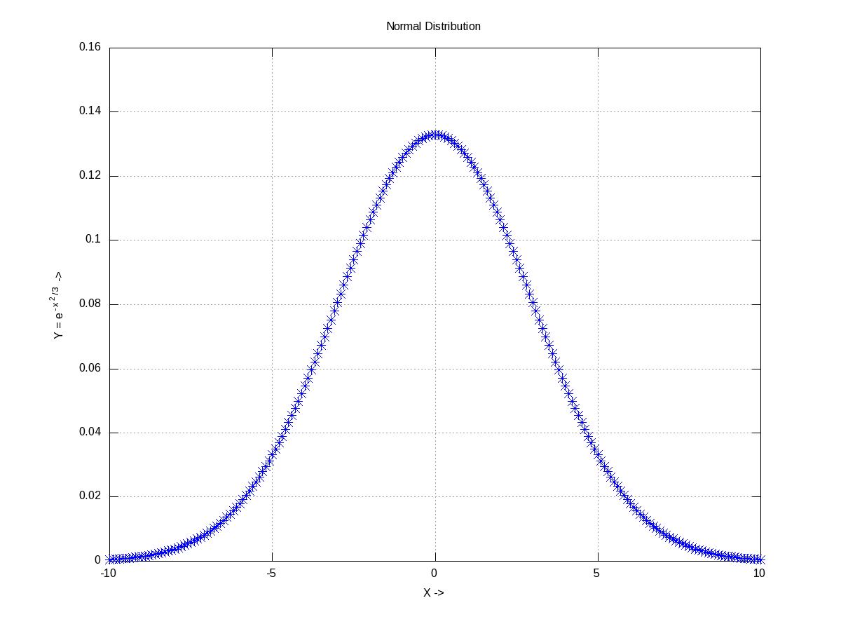
Already got scared by the name itself. Don’t worry. Moments basically mean the various kinds of averages, median, modes, etc. To understand them, let’s take some random data set, which may be generated using any of the various distributions. Let’s take the most “natural” normal distribution – yes the bell-shaped one. Figure 19 shows one centered around 0 (the mean) with a spread of 3 (the standard deviation), generated using normpdf(), as cited below. Note that octave has a whole set of all such functions.

$ octave -qf
octave:1> X = -10:0.1:10;
octave:2> Y = normpdf(X, 0, 3); # Normal Density Function
octave:3> plot(X, Y, "b*");
octave:4> xlabel("X ->");
octave:5> ylabel("Y = e^{-{x^2}/3} ->");
octave:6> title("Normal Distribution");
octave:7> grid("on");
octave:8>
Figure 19: Normal distribution with mean = 0, std = 3

Figure 19: Normal distribution with mean = 0, std = 3

If we take all the infinite points on this curve, would get a mean of 0 and a standard deviation of 3. But that’s not practical. So, let’s pick, say 10 random points from it. normrnd(m, s, 10, 1) provides the same in a 10×1 vector, following the normal distribution of mean m & standard deviation s. And then, mean() & std() give the mean and standard deviation, respectively. mean() could be of three types: Ordinary (arithmetic) mean (“a”), Geometric mean (“g”), Harmonic mean (“h”).

$ octave -qf
octave:1> Y = normrnd(0, 3, 10, 1) # m=0; s=3; 10x1 vector
Y =

  -2.33218
  -3.16866
   3.41991
  -2.27566
  -1.45403
   7.79691
   2.12849
   2.32727
  -5.37920
  -0.63447
octave:2> mean(Y)
ans =  0.042839
octave:3> mean(Y, "h")
ans =  -4.3226
octave:4> std(Y)
ans =  3.8662
octave:5> median(Y)
ans = -1.0442
octave:6> cov(Y, Y)
ans =  14.947
octave:7> cor(Y, Y)
ans =  1
octave:8>

Among many other moments, the four common ones are: 1) median() gets the middle most element in the sorted arrangement of data; 2) mode() gets the most frequently occurring data point; 3) cov() gives the variance between two set of data points, i.e. the covariance; 4) cor() gives the relation between two set of data points, i.e. the correlation ranging from -1 to 1. Correlation of 1 indicating they are completely related, 0 indicating totally unrelated, and a -1 indicating related completely but in an opposite sense.

Visualizing the probabilities

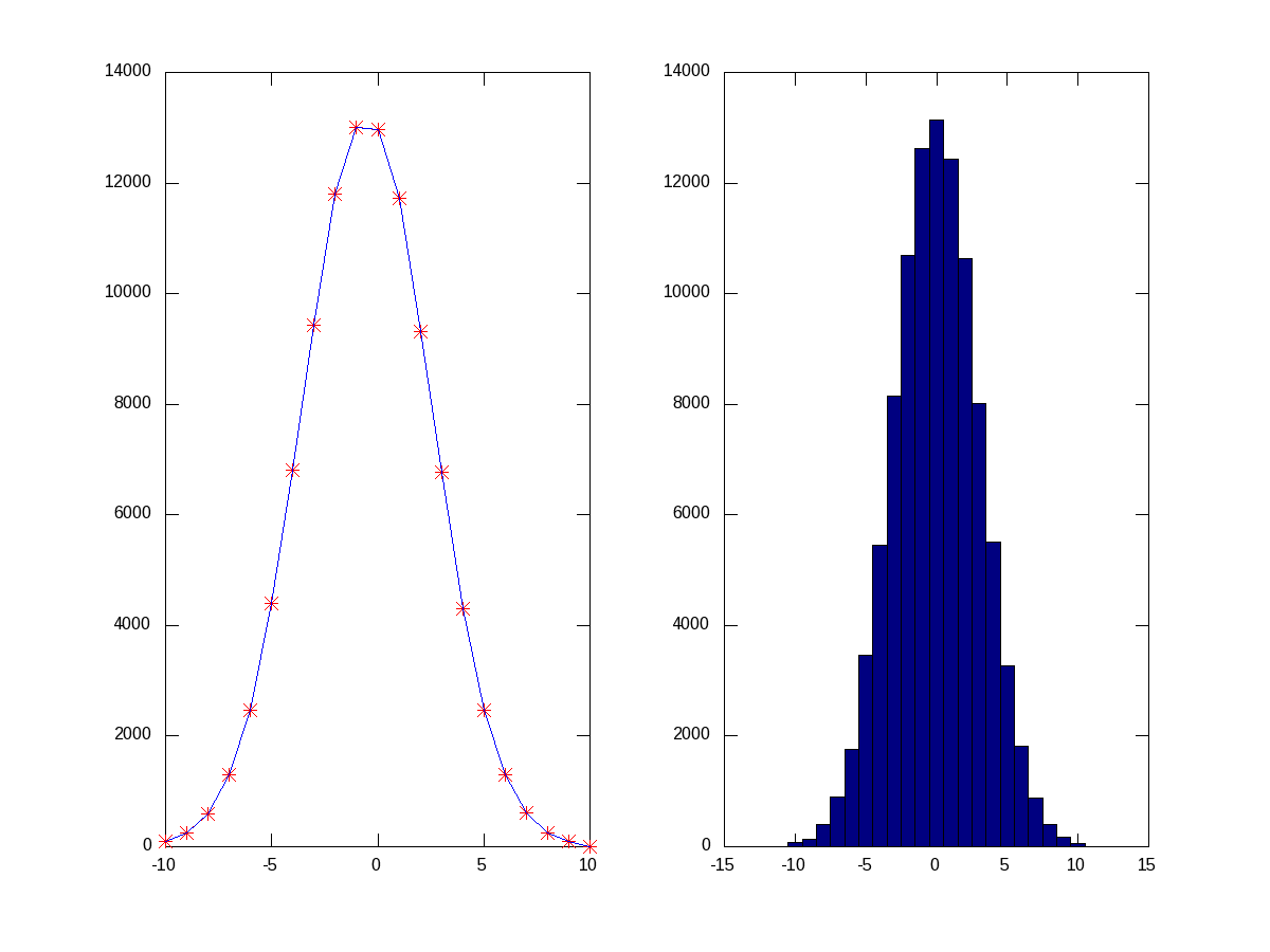
Random numbers are a beautiful example of probabilities. They occur as per their probabilities decided by the probability density function (PDF) they follow. Let’s visualize that using a live example. So again, as in the above example, let’s take some random numbers following the normal distribution. But, this time we’ll take a lot more points, say 1,00,000 points, so that we can actually see them following the bell-shape. But still, we are not having infinite points to give the continuous bell. So, what we have to do is collect the random points around some pre-designated buckets of fixed ranges. That is what we call a histogram. histc() does exactly that, returning the number of points in each of the buckets, which we can then plot to see our bell. Another function hist(), does all those in a more beautiful way. Figure 20 shows the two plots, for which the code follows:

$ octave -qf
octave:1> Y=normrnd(0, 3, 100000, 1); # 1 lakh random points
octave:2> B=-10:1:10; # Bucket edges -10, -9, ..., 10, i.e. 21 buckets
octave:3> N=histc(Y, B);
octave:4> subplot(1, 2, 1);
octave:5> plot(B, N, "r*", B, N, "b-");
octave:6> subplot(1, 2, 2);
octave:7> hist(Y, B); # More beautiful boxy plot
octave:8>
Figure 20: Histograms of normal distributed random points

Figure 20: Histograms of normal distributed random points

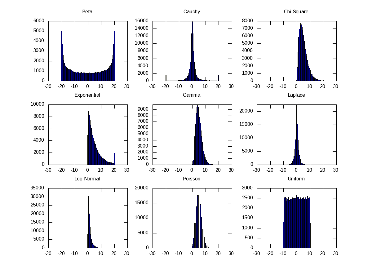
Similarly, if we use other PDFs, we would see similar histograms for them as well. Figure 21 shows nine such others, namely Beta (with alpha = beta = 0.5), Cauchy, Chi-Square, Exponential, Gamma, Laplace, Log Normal, Poisson, Uniform, using their respective functions, as shown in the code below:

octave:1> B=-20:0.5:20;
octave:2> subplot(3, 3, 1);
octave:3> hist(40*(betarnd(0.5, 0.5, 100000, 1) - 0.5), B);
octave:4> title("Beta");
octave:5> subplot(3, 3, 2);
octave:6> hist(cauchy_rnd(0, 1, 100000, 1), B);
octave:7> title("Cauchy");
octave:8> subplot(3, 3, 3);
octave:9> hist(chi2rnd(5, 100000, 1), B);
octave:10> title("Chi Square");
octave:11> subplot(3, 3, 4);
octave:12> hist(exprnd(5, 100000, 1), B);
octave:13> title("Exponential");
octave:14> subplot(3, 3, 5);
octave:15> hist(gamrnd(5, 1, 100000, 1), B);
octave:16> title("Gamma");
octave:17> subplot(3, 3, 6);
octave:18> hist(laplace_rnd(100000, 1), B);
octave:19> title("Laplace");
octave:20> subplot(3, 3, 7);
octave:21> hist(lognrnd(0, 1, 100000, 1), B);
octave:22> title("Log Normal");
octave:23> subplot(3, 3, 8);
octave:24> hist(poissrnd(5, 100000, 1), B);
octave:25> title("Poisson");
octave:26> subplot(3, 3, 9);
octave:27> hist(unifrnd(-10, 10, 100000, 1), B);
octave:28> title("Uniform");
octave:29>
Figure 21: Histograms of probability density functions

Figure 21: Histograms of probability density functions

Miscellaneous helpers

Apart from the standard ones, discussed so far, there are quite a few miscellaneous useful functions provided by octave. Here are a few:

  • perms() – Generates the n! permutations of the data points
  • values() – Sorts the data into non-repeating ascending order
  • range() – Returns the difference between the maximum and the minimum data points

Here follows a demonstration:

$ octave -qf
octave:1> perms([0 1 2])
ans =

   0   1   2
   1   0   2
   0   2   1
   1   2   0
   2   0   1
   2   1   0

octave:2> values([1 4 -9 -7 0 -6 12 -90])
ans =

  -90
   -9
   -7
   -6
    0
    1
    4
   12

octave:3> range([1 4 -9 -7 0 -6 12 -90])
ans =  102
octave:4>

What’s next?

Till date, in all our mathematical explorations, we have been always dealing with numbers. Ya! So big deal – anyways mathematics is about numbers, only. Not really. Many a times, we come across scenarios, where we would like to solve something symbolically or analytically, and then use numbers only at the end. Such things would not be possible with any of the OSS tools, we have discussed till now. But, yes there are such tools. One such is Maxima. And that’s where we are headed to next.

Fourteenth Article >>

   Send article as PDF   

USB Drivers in Linux (Continued)

This twelfth article, which is part of the series on Linux device drivers, gets you further with writing your first USB driver in Linux – a continuation from the previous article.

<< Eleventh Article

Pugs continued, “Let’s build upon the USB device driver coded in our previous session, using the same handy JetFlash pen drive from Transcend with vendor id 0x058f and product id 0x6387. For that, we would dig further into the USB protocol and then convert the learning into code.”

USB endpoints and their types

Depending on the type and attributes of information to be transferred, a USB device may have one or more endpoints, each belonging to one of the following four categories:

  • Control – For transferring control information. Examples include resetting the device, querying information about the device, etc. All USB devices always have the default control endpoint point zero.
  • Interrupt – For small and fast data transfer, typically of up to 8 bytes. Examples include data transfer for serial ports, human interface devices (HIDs) like keyboard, mouse, etc.
  • Bulk – For big but comparatively slow data transfer. A typical example is data transfers for mass storage devices.
  • Isochronous – For big data transfer with bandwidth guarantee, though data integrity may not be guaranteed. Typical practical usage examples include transfers of time-sensitive data like of audio, video, etc.

Additionally, all but control endpoints could be “in” or “out”, indicating its direction of data transfer. “in” indicates data flow from USB device to the host machine and “out” indicates data flow from the host machine to USB device. Technically, an endpoint is identified using a 8-bit number, most significant bit (MSB) of which indicates the direction – 0 meaning out, and 1 meaning in. Control endpoints are bi-directional and the MSB is ignored.

Figure 19: USB's proc window snippet

Figure 19: USB’s proc window snippet

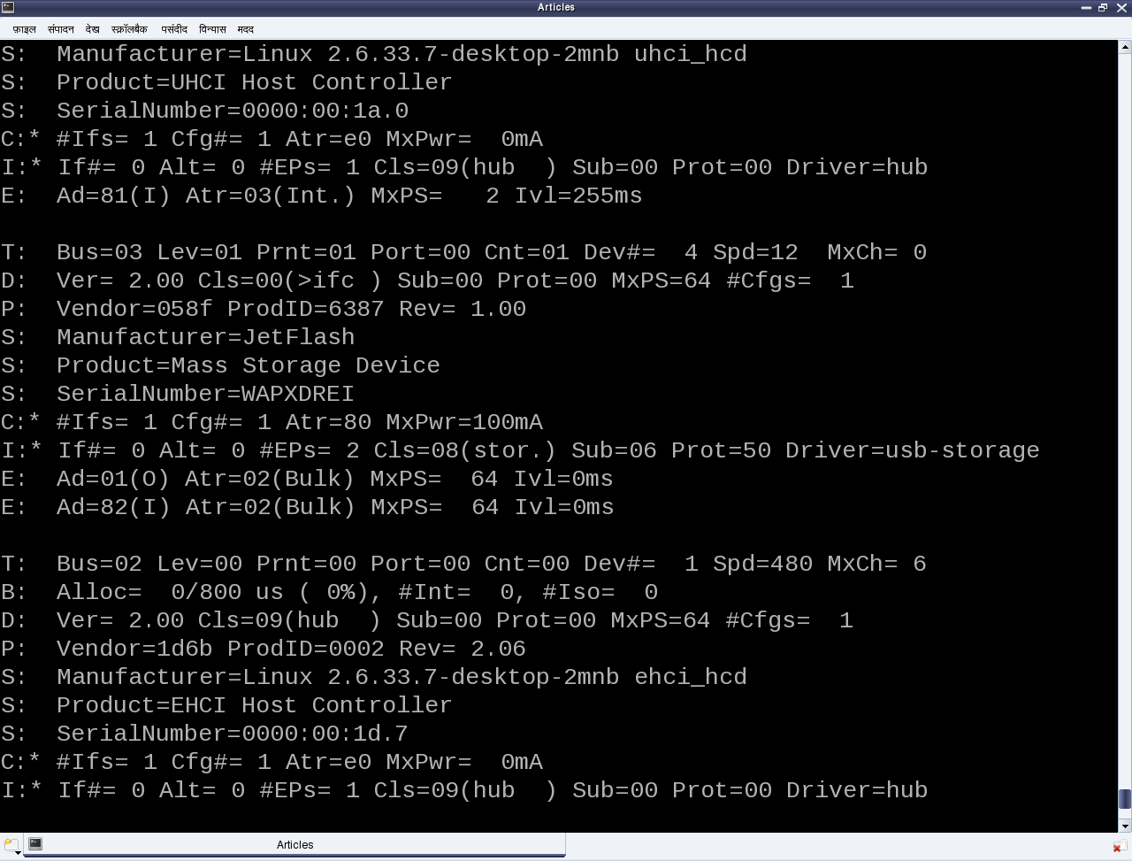
Figure 19 shows a typical snippet of USB device specifications for devices connected on a system. To be specific, the “E: ” lines in the figure shows example of an interrupt endpoint of a UHCI Host Controller and two bulk endpoints of the pen drive under consideration. Also, the endpoint numbers (in hex) are respectively 0x81, 0x01, 0x82. The MSB of the first and third being 1 indicating “in” endpoints, represented by “(I)” in the figure. Second one is an “(O)” for the “out” endpoint. “MaxPS” specifies the maximum packet size, i.e. the data size that can be transferred in a single go. Again as expected, for the interrupt endpoint it is 2 (<= 8), and 64 for the bulk endpoints. “Ivl” specifies the interval in milliseconds to be given between two consecutive data packet transfers for proper transfer and is more significant for the interrupt endpoints.

Decoding a USB device section

As we have just discussed the “E: ” line, it is right time to decode the relevant fields of others as well. In short, these lines in a USB device section gives the complete overview of the USB device as per the USB specifications, as discussed in our previous article. Refer back to Figure 19. The first letter of the first line of every device section is a “T” indicating the position of the device in the USB tree, uniquely identified by the triplet <usb bus number, usb tree level, usb port>. “D” represents the device descriptor containing at least the device version, device class/category, and the number of configurations available for this device. There would be as many “C” lines as the number of configurations, typically one. “C” represents the configuration descriptor containing its index, device attributes in this configuration, maximum power (actually current) the device would draw in this configuration, and the number of interfaces under this configuration. Depending on that there would be at least that many “I” lines. There could be more in case of an interface having alternates, i.e. same interface number but with different properties – a typical scenario for web-cams.

“I” represents the interface descriptor with its index, alternate number, functionality class/category of this interface, driver associated with this interface, and the number of endpoints under this interface. The interface class may or may not be same as that of the device class. And depending on the number of endpoints, there would be as many “E” lines, details of which have already been discussed above. The “*” after the “C” & “I” represents the currently active configuration and interface, respectively. “P” line provides the vendor id, product id, and the product revision. “S” lines are string descriptors showing up some vendor specific descriptive information about the device.

“Peeping into /proc/bus/usb/devices is good to figure out whether a device has been detected or not and possibly to get the first cut overview of the device. But most probably this information would be required in writing the driver for the device as well. So, is there a way to access it using ‘C’ code?”, asked Shweta. “Yes definitely, that’s what I am going to tell you next. Do you remember that as soon as a USB device is plugged into the system, the USB host controller driver populates its information into the generic USB core layer? To be precise, it puts that into a set of structures embedded into one another, exactly as per the USB specifications”, replied Pugs. The following are the exact data structures defined in <linux/usb.h> – ordered here in reverse for flow clarity:

struct usb_device
{
	...
	struct usb_device_descriptor descriptor;
	struct usb_host_config *config, *actconfig;
	...
};
struct usb_host_config
{
	struct usb_config_descriptor desc;
	...
	struct usb_interface *interface[USB_MAXINTERFACES];
	...
};
struct usb_interface
{
	struct usb_host_interface *altsetting /* array */, *cur_altsetting;
	...
};
struct usb_host_interface
{
	struct usb_interface_descriptor desc;
	struct usb_host_endpoint *endpoint /* array */;
	...
};
struct usb_host_endpoint
{
	struct usb_endpoint_descriptor  desc;
	...
};

So, with access to the struct usb_device handle for a specific device, all the USB specific information about the device can be decoded, as shown through the /proc window. But how to get the device handle? In fact, the device handle is not available directly in a driver, rather the per interface handles (pointers to struct usb_interface) are available, as USB drivers are written for device interfaces rather than the device as a whole. Recall that the probe & disconnect callbacks, which are invoked by USB core for every interface of the registered device, have the corresponding interface handle as their first parameter. Refer the prototypes below:

int (*probe)(struct usb_interface *interface, const struct usb_device_id *id);
void (*disconnect)(struct usb_interface *interface);

So with the interface pointer, all information about the corresponding interface can be accessed. And to get the container device handle, the following macro comes to rescue:

struct usb_device device = interface_to_usbdev(interface);

Adding these new learning into the last month’s registration only driver, gets the following code listing (pen_info.c):

#include <linux/module.h>
#include <linux/kernel.h>
#include <linux/usb.h>

static struct usb_device *device;

static int pen_probe(struct usb_interface *interface, const struct usb_device_id *id)
{
	struct usb_host_interface *iface_desc;
	struct usb_endpoint_descriptor *endpoint;
	int i;

	iface_desc = interface->cur_altsetting;
	printk(KERN_INFO "Pen i/f %d now probed: (%04X:%04X)\n",
			iface_desc->desc.bInterfaceNumber,
			id->idVendor, id->idProduct);
	printk(KERN_INFO "ID->bNumEndpoints: %02X\n",
			iface_desc->desc.bNumEndpoints);
	printk(KERN_INFO "ID->bInterfaceClass: %02X\n",
			iface_desc->desc.bInterfaceClass);

	for (i = 0; i < iface_desc->desc.bNumEndpoints; i++)
	{
		endpoint = &iface_desc->endpoint[i].desc;

		printk(KERN_INFO "ED[%d]->bEndpointAddress: 0x%02X\n",
				i, endpoint->bEndpointAddress);
		printk(KERN_INFO "ED[%d]->bmAttributes: 0x%02X\n",
				i, endpoint->bmAttributes);
		printk(KERN_INFO "ED[%d]->wMaxPacketSize: 0x%04X (%d)\n",
				i, endpoint->wMaxPacketSize,
				endpoint->wMaxPacketSize);
	}

	device = interface_to_usbdev(interface);
	return 0;
}

static void pen_disconnect(struct usb_interface *interface)
{
	printk(KERN_INFO "Pen i/f %d now disconnected\n",
			interface->cur_altsetting->desc.bInterfaceNumber);
}

static struct usb_device_id pen_table[] =
{
	{ USB_DEVICE(0x058F, 0x6387) },
	{} /* Terminating entry */
};
MODULE_DEVICE_TABLE (usb, pen_table);

static struct usb_driver pen_driver =
{
	.name = "pen_info",
	.probe = pen_probe,
	.disconnect = pen_disconnect,
	.id_table = pen_table,
};

static int __init pen_init(void)
{
	return usb_register(&pen_driver);
}

static void __exit pen_exit(void)
{
	usb_deregister(&pen_driver);
}

module_init(pen_init);
module_exit(pen_exit);

MODULE_LICENSE("GPL");
MODULE_AUTHOR("Anil Kumar Pugalia <email@sarika-pugs.com>");
MODULE_DESCRIPTION("USB Pen Info Driver");

Then, the usual steps for any Linux device driver may be repeated, along with the pen drive steps:

  • Build the driver (pen_info.ko file) by running make.
  • Load the driver using insmod pen_info.ko.
  • Plug-in the pen drive (after making sure that usb-storage driver is not already loaded).
  • Unplug-out the pen drive.
  • Check the output of dmesg for the logs.
  • Unload the driver using rmmod pen_info.

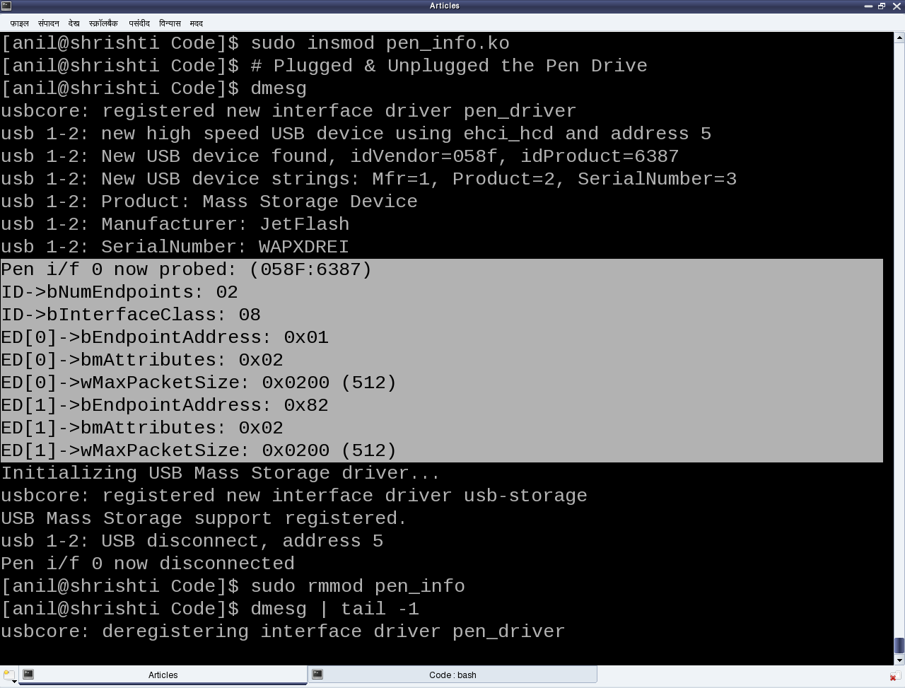
Figure 22 shows a snippet of the above steps on Pugs’ system. Remember to ensure (in the output of cat /proc/bus/usb/devices) that the usual usb-storage driver is not the one associated with the pen drive interface, rather it should be the pen_info driver.

Figure 22: Output of dmesg

Figure 22: Output of dmesg

Summing up

Before taking another break, Pugs shared two of the many mechanisms for a driver to specify its device to the USB core, using the struct usb_device_id table. First one is by specifying the <vendor id, product id> pair using the USB_DEVICE() macro (as done above), and the second one is by specifying the device class/category using the USB_DEVICE_INFO() macro. In fact, many more macros are available in <linux/usb.h> for various combinations. Moreover, multiple of these macros could be specified in the usb_device_id table (terminated by a null entry), for matching with any one of the criteria, enabling to write a single driver for possibly many devices.

“Earlier you mentioned writing multiple drivers for a single device, as well. Basically, how do we selectively register or not register a particular interface of a USB device?”, queried Shweta. “Sure. That’s next in line of our discussion, along with the ultimate task in any device driver – the data transfer mechanisms” replied Pugs.

Thirteenth Article >>

Notes

  1. Make sure that you replace the vendor id & device id in the above code examples by the ones of your pen drive.
  2. One may wonder, as how does the usb-storage get autoloaded. The answer lies in the module autoload rules written down in the file /lib/modules/<kernel_version>/modules.usbmap. If you are an expert, you may comment out the corresponding line, for it to not get autoloaded. And uncomment it back, once you are done with your experiments.
  3. In latest distros, you may not find the detailed description of the USB devices using cat /proc/bus/usb/devices, as the /proc/bus/usb/ itself has been deprecated. You can find the same detailed info using cat /sys/kernel/debug/usb/devices – though you may need root permissions for the same. Also, if you do not see any file under /sys/kernel/debug (even as root), then you may have to first mount the debug filesystem, as follows: mount -t debugfs none /sys/kernel/debug
   Send article as PDF   

Figures, Graphs, and Plots in Octave

This twelfth article of the mathematical journey through open source, shows the mathematical visualization in octave.

<< Eleventh Article

Mathematics is incomplete without visualization, without drawing the results, and without plotting the graphs. octave uses the powerful gnuplot as the backend of its plotting functionality. And in the frontend provides various plotting functions. Let’s look at the most beautiful ones.

Basic 2D Plotting

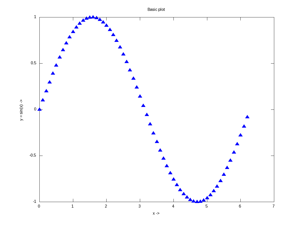
The most basic plotting is using the plot() function, which takes the Cartesian x & y values. Additionally, you may pass, as how to plot, i.e. as points or lines, their style, their colour, label, etc. Supported point styles are: +, *, o, x, ^, and lines are represented by -. Supported colours are: k (black), r (red), g (green), b (blue), y (yellow), m (magenta), c (cyan), w (white). With this background, here is how you plot a sine curve, and Figure 12 shows the plot.

$ octave -qf
octave:1> x = 0:0.1:2*pi;
octave:2> y = sin(x);
octave:3> plot(x, y, "^b");
octave:4> xlabel("x ->");
octave:5> ylabel("y = sin(x) ->");
octave:6> title("Basic plot");
octave:7>
Figure 12: Basic plotting in octave

Figure 12: Basic plotting in octave

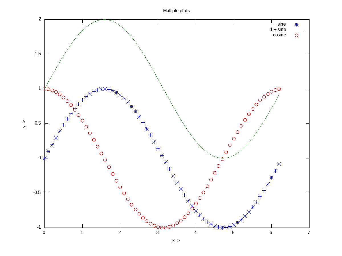
xlabel(), and ylabel() adds the corresponding labels, and title() adds the title. Multiple plots can be done on the same axis as follows, and Figure 13 shows the plots. Note the usage of legend() to mark the multiple plots.

$ octave -qf
octave:1> x = 0:0.1:2*pi;
octave:2> plot(x, sin(x), "*", x, 1 + sin(x), "-", x, cos(x), "o");
octave:3> xlabel("x ->");
octave:4> ylabel("y ->");
octave:5> legend("sine", "1 + sine", "cosine");
octave:6> title("Multiple plots");
octave:7>
Figure 13: Multiple plots on the same axis

Figure 13: Multiple plots on the same axis

Advanced 2D Figures

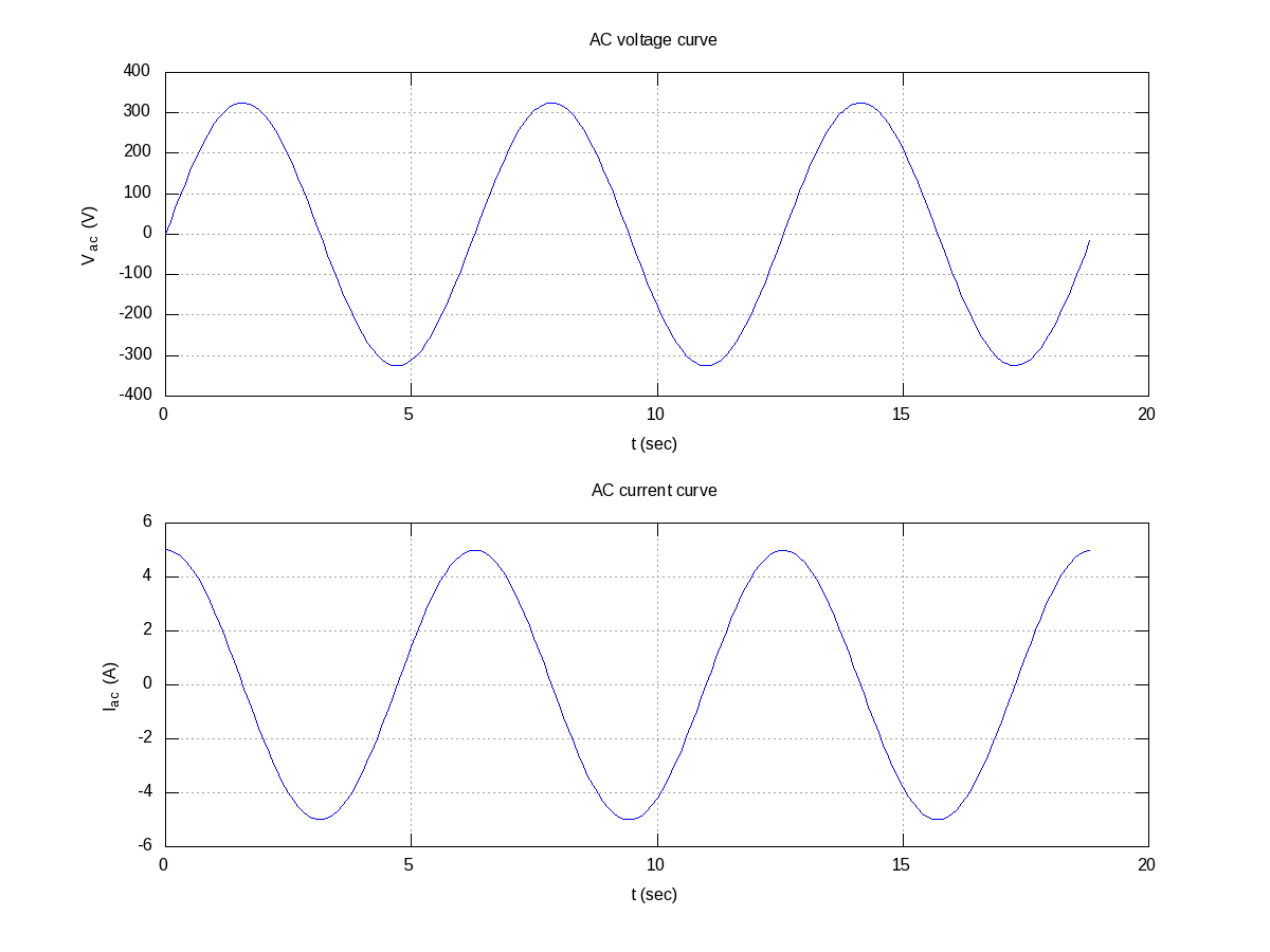
Now, if we want to have the multiple graphs on the same sheet but with different axes as shown in Figure 14, here is how to do that:

octave:1> t = 0:0.1:6*pi;
octave:2> subplot(2, 1, 1);
octave:3> plot(t, 325 * sin(t));
octave:4> xlabel("t (sec)");
octave:5> ylabel("V_{ac} (V)");
octave:6> title("AC voltage curve");
octave:7> grid("on");
octave:8> subplot(2, 1, 2);
octave:9> plot(t, 5 * cos(t));
octave:10> xlabel("t (sec)");
octave:11> ylabel("I_{ac} (A)");
octave:12> title("AC current curve");
octave:13> grid("on");
octave:14> print("-dpng", "multiple_plots_on_a_sheet.png");
octave:15>
Figure 14: Multiple plots on a sheet

Figure 14: Multiple plots on a sheet

Note the usage of subplot(), taking the matrix dimensions (row, column) and the plot number to create the matrix of plots. In the example above, it created a 2×1 matrix of plots. As add-ons, we have used the grid(“on”) to show up the dotted grid lines, and print() to save the generated figure as a .png file.

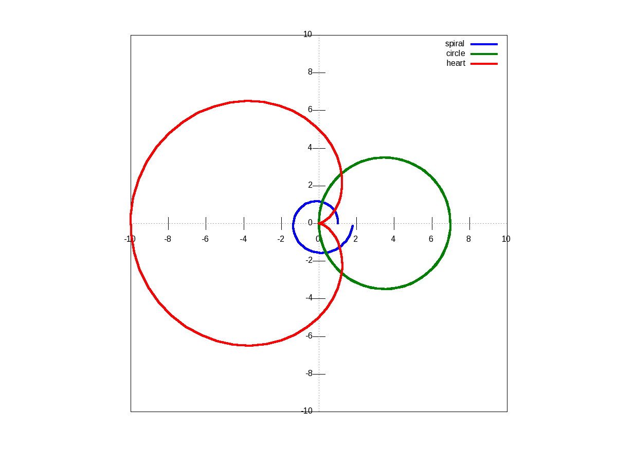
It is not always easy to plot everything in Cartesian co-ordinates, or rather many things are easier to plot in polar co-ordinates, e.g. a spiral, circle, heart, etc. The following code & Figure 15 shows a few such examples. Shown along with is a technique of modifying the figure properties, after drawing the figure using the set() function. Here it modifies the line thickness.

octave:1> th = 0:0.1:2*pi;
octave:2> r1 = 1.1 .^ th;
octave:3> r2 = 7 * cos(th);
octave:4> r3 = 5 * (1 - cos(th));
octave:5> r = [r1; r2; r3];
octave:6> ph = polar(th, r, "-");
octave:7> set(ph, "LineWidth", 4);
octave:8> legend("spiral", "circle", "heart");
octave:9>
Figure 15: Polar plots

Figure 15: Polar plots

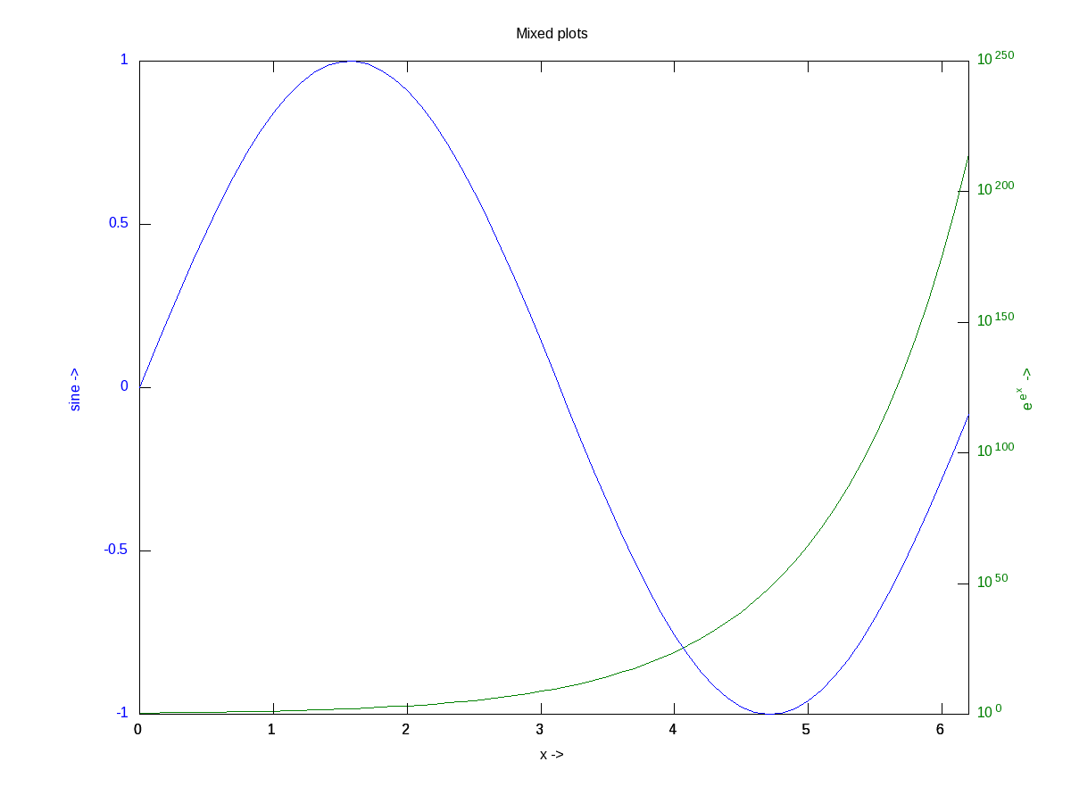
There are many other possible ways of drawing various interesting 2-D figures for all kind of mathematical & scientific requirements. So, before closing on 2-D plotting, let’s look into just one more often needed drawing – plotting with log axis, and more over with two y-axes on a single plot. The function for that is plotyy(). Note the plotyy() calling the corresponding function pointers @plot, @semilogy passed to it, in the following code segment. Figure 16 shows the output.

octave:1> x = 0:0.1:2*pi;
octave:2> y1 = sin(x);
octave:3> y2 = exp(exp(x));
octave:4> ax = plotyy(x, y1, x, y2, @plot, @semilogy);
octave:5> xlabel("x ->");
octave:6> ylabel(ax(1), "sine ->");
octave:7> ylabel(ax(2), "e^{e^x} ->");
octave:8> title("Mixed plots");
octave:9>
Figure 16: Mixed plots with semi log axis

Figure 16: Mixed plots with semi log axis

3D Visualization

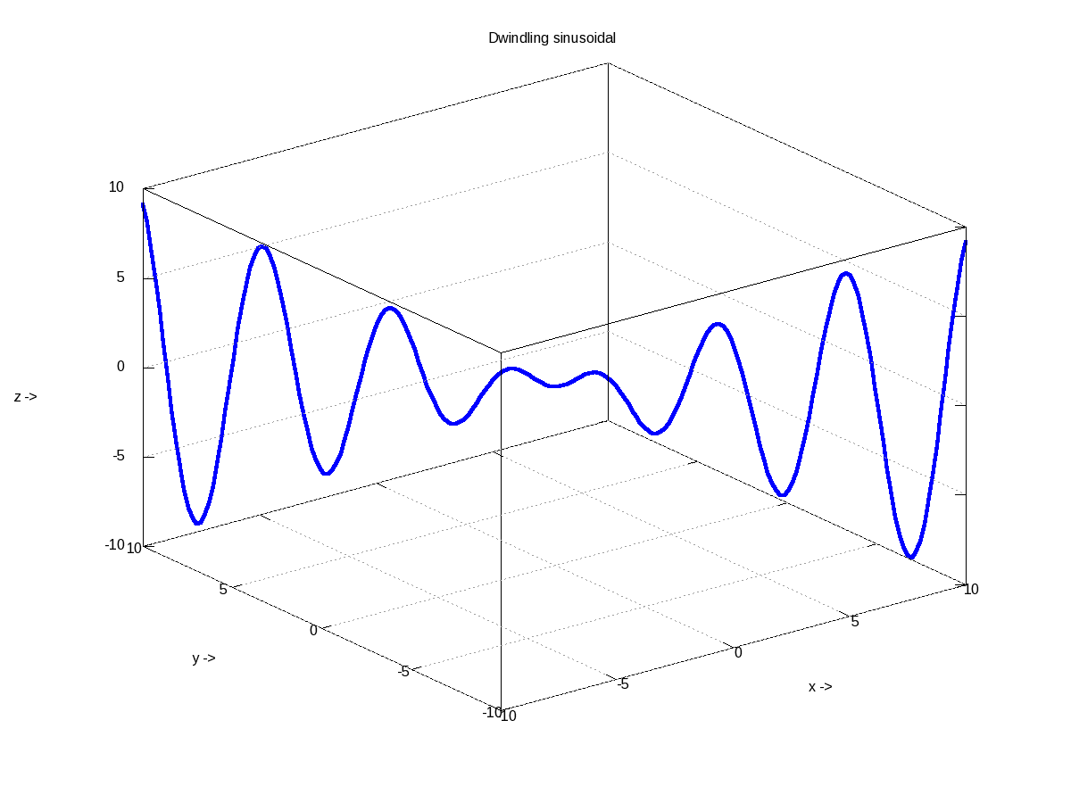
And finally, let’s do some 3-D plotting. plot3() is the simplest octave function to do a simple 3-D drawing, taking the set of (x, y, z) points. Here’s the sample code to draw the dwindling sinusoidal curve shown in Figure 17:

octave:1> x = -10:0.1:10;
octave:2> y = 10:-0.1:-10;
octave:3> z = x .* sin(x - y); 
octave:4> plot3(x, y, z, "-", "LineWidth", 4); 
octave:5> xlabel("x ->");
octave:6> ylabel("y ->");
octave:7> zlabel("z ->");
octave:8> title("Dwindling sinusoidal");
octave:9> grid("on");
octave:10>
Figure 17: 3-D plot of a dwindling sinusoidal

Figure 17: 3-D plot of a dwindling sinusoidal

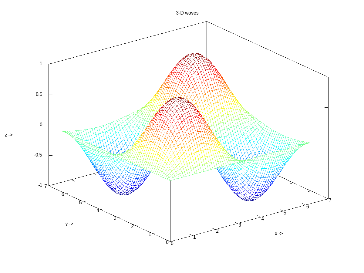
In case, we want to plot the values of a 2-D matrix against its indices (x, y), it could be done using mesh(), one of the many other 3-D plotting functions. Figure 18 shows the same, created using the following code:

octave:1> x = 0:0.1:2*pi;
octave:2> y = 0:0.1:2*pi;
octave:3> z = sin(x)' * sin(y);
octave:4> mesh(x, y, z); 
octave:5> xlabel("x ->");
octave:6> ylabel("y ->");
octave:7> zlabel("z ->");
octave:8> title("3-D waves");
octave:9>
Figure 18: 3-D waves

Figure 18: 3-D waves

What’s next?

Hope you enjoyed the colours of drawing. Next, we would look into octave from a statisticians perspective.

Thirteenth Article >>

   Send article as PDF   

USB Drivers in Linux

This eleventh article, which is part of the series on Linux device drivers, gets you started with writing your first USB driver in Linux.

<< Tenth Article

Pugs’ pen drive was the device, Shweta was playing with, when both of them sat down to explore the world of USB drivers in Linux. The fastest way to get hang of one, the usual Pugs’ way, was to pick up a USB device and write a driver for it to experiment with. So, they chose pen drive aka USB stick, available at hand. It was JetFlash from Transcend with vendor ID 0x058f and product ID 0x6387.

USB device detection in Linux

Whether a driver of a USB device is there or not on a Linux system, a valid USB device would always get detected at the hardware and kernel spaces of a USB-enabled Linux system. A valid USB device is a device designed and detected as per USB protocol specifications. Hardware space detection is done by the USB host controller – typically a native bus device, e.g. a PCI device on x86 systems. The corresponding host controller driver would pick and translate the low-level physical layer information into higher level USB protocol specific information. The USB protocol formatted information about the USB device is then populated into the generic USB core layer (usbcore driver) in the kernel space, thus enabling the detection of a USB device in the kernel space, even without having its specific driver.

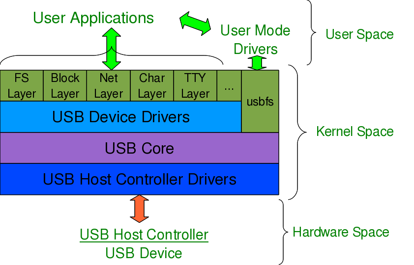
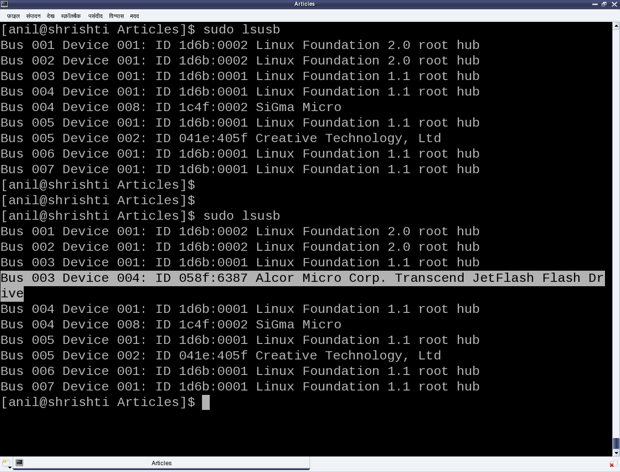
After this, it is up to the various drivers, interfaces, and applications (which are dependent on the various Linux distributions), to have the user space view of the detected devices. Figure 17 shows a top to bottom view of USB subsystem in Linux. A basic listing of all detected USB devices can be obtained using the lsusb command, as root. Figure 18 shows the same, without and with the pen drive being inserted into the system. A -v option to lsusb provides detailed information. In many Linux distributions like Mandriva, Fedora, … usbfs driver is loaded as part of the default configuration. This enables the detected USB device details to be viewed in a more techno-friendly way through the /proc window using cat /proc/bus/usb/devices. Figure 19 shows a typical snippet of the same, clipped around the pen drive specific section. The complete listing basically contains such sections, each for one of the valid USB devices detected on the Linux system.

Figure 17: USB subsystem in Linux

Figure 17: USB subsystem in Linux

Figure 18: Output of lsusb

Figure 18: Output of lsusb

Figure 19: USB's proc window snippet

Figure 19: USB’s proc window snippet

Decoding a USB device section

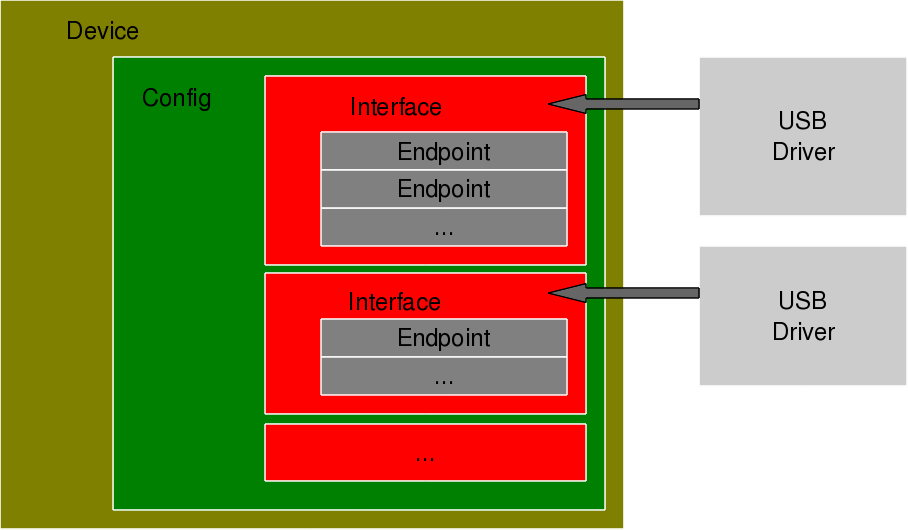
To further decode these sections, a valid USB device needs to be understood first. All valid USB devices contain one or more configurations. A configuration of a USB device is like a profile, where the default one is the commonly used one. As such, Linux supports only one configuration per device – the default one. For every configuration, the device may have one or more interfaces. An interface corresponds to the functionality provided by the device. There would be as many interfaces as the number of independent functionalities provided by the device. So, say an MFD (multi-function device) USB printer can do printing, scanning, and faxing, then it most likely would have at least three interfaces – one for each of the functionalities. So, unlike other device drivers, a USB device driver is typically associated/written per interface, rather than the device as a whole – meaning one USB device may have multiple device drivers. Though definitely one interface can have a maximum of one driver only.

Moreover, it is okay and common to have a single USB device driver for all the interfaces of a USB device. The “Driver=…” entry in the proc window output (Figure 19) shows the interface is to driver mapping – a “(none)” indicating no associated driver. For every interface, there would be one or more end points. An endpoint is like a pipe for transferring information either into or from the interface of the device, depending on the functionality. Depending on the type of information, the endpoints have four types:

  • Control
  • Interrupt
  • Bulk
  • Isochronous

As per USB protocol specification, all valid USB devices have an implicit special control endpoint zero, the only bi-directional endpoint. Figure 20 shows the complete pictorial representation of a valid USB device, based on the above explanation.

Coming back to the USB device sections (Figure 19), the first letter on each line represents the various parts of the USB device specification just explained. For example, D for device, C for configuration, I for interface, E for endpoint, etc. Details about them and various others are available under the kernel source Documentation/usb/proc_usb_info.txt

Figure 20: USB device overview

Figure 20: USB device overview

The USB pen drive driver registration

“Seems like there are so many things to know about the USB protocol to be able to write the first USB driver itself – device configuration, interfaces, transfer pipes, their four types, and so many other symbols like T, B, S, … under a USB device specification”, sighed Shweta. “Yes, but don’t you worry – all these can be talked in detail, later. Let’s do the first thing first – get our pen drive’s interface associated with our USB device driver (pen_register.ko)”, consoled Pugs. Like any other Linux device driver, here also we need the constructor and the destructor – basically the same driver template that has been used for all the drivers. Though the content would vary as this is a hardware protocol layer driver, i.e. a horizontal driver unlike a character driver, which was one of the vertical drivers, discussed so far. And the difference would be that instead of registering with & unregistering from VFS, here we would do that with the corresponding protocol layer – the USB core in this case; instead of providing a user space interface like a device file, it would get connected with the actual device in the hardware space. The USB core APIs for the same are as follows (prototyped in <linux/usb.h>):

int usb_register(struct usb_driver *driver);
void usb_deregister(struct usb_driver *);

As part of the usb_driver structure, the fields to be provided are the driver’s name, ID table for auto-detecting the particular device and the 2 callback functions to be invoked by USB core during hot-plugging and hot-removal of the device, respectively. Putting it all together, pen_register.c would look like:

#include <linux/module.h>
#include <linux/kernel.h>
#include <linux/usb.h>

static int pen_probe(struct usb_interface *interface, const struct usb_device_id *id)
{
	printk(KERN_INFO "Pen drive (%04X:%04X) plugged\n", id->idVendor,
								id->idProduct);
	return 0;
}

static void pen_disconnect(struct usb_interface *interface)
{
	printk(KERN_INFO "Pen drive removed\n");
}

static struct usb_device_id pen_table[] =
{
	{ USB_DEVICE(0x058F, 0x6387) },
	{} /* Terminating entry */
};
MODULE_DEVICE_TABLE (usb, pen_table);

static struct usb_driver pen_driver =
{
	.name = "pen_driver",
	.id_table = pen_table,
	.probe = pen_probe,
	.disconnect = pen_disconnect,
};

static int __init pen_init(void)
{
	return usb_register(&pen_driver);
}

static void __exit pen_exit(void)
{
	usb_deregister(&pen_driver);
}

module_init(pen_init);
module_exit(pen_exit);

MODULE_LICENSE("GPL");
MODULE_AUTHOR("Anil Kumar Pugalia <email@sarika-pugs.com>");
MODULE_DESCRIPTION("USB Pen Registration Driver");

Then, the usual steps for any Linux device driver may be repeated:

  • Build the driver (.ko file) by running make
  • Load the driver using insmod
  • List the loaded modules using lsmod
  • Unload the driver using rmmod

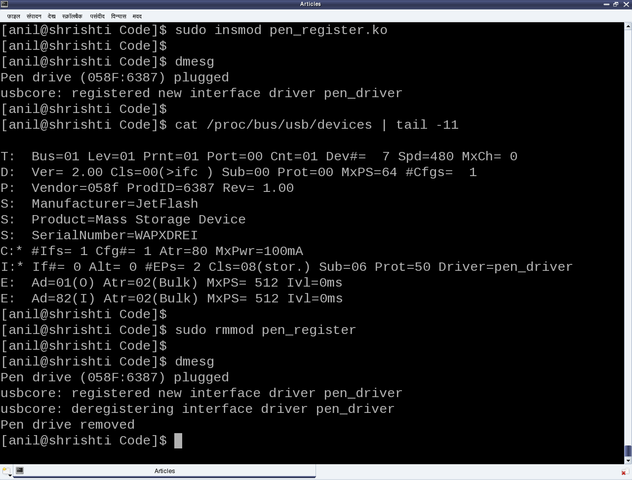
But surprisingly the results wouldn’t be as expected. Check for dmesg and the proc window to see the various logs and details. Not because USB driver is different from a character driver. But there’s a catch. Figure 19 shows that the pen drive has one interface (numbered 0), which is already associated with the usual usb-storage driver. Now, in order to get our driver associated with that interface, we need to unload the usb-storage driver (i.e. rmmod usb-storage) after plugging in the pen drive, and then load our driver. Once this sequence is followed, the results would be as expected. Figure 21 shows a glimpse of the possible logs and proc window snippet. Repeat hot-plugging in and hot-plugging out the pen drive to observe the probe and disconnect calls in action – but don’t forget unloading the usb-storage driver, every time you plug in the pen driver.

Figure 21: Pen driver in action

Figure 21: Pen driver in action

Summing up

“Finally!!! Something into action.”, relieved Shweta. “But seems like there are so many things around (like the device ID table, probe, disconnect, …), yet to be assimilated and understood to get a complete USB device driver, in place”, she continued. “Yes, you are right. Let’s take them one by one, with breaks”, replied Pugs taking a stretching break.

Twelfth Article >>

Notes

  1. Make sure that you replace the vendor id & device id in the above code examples by the ones of your pen drive.
  2. One may wonder, as how does the usb-storage get autoloaded. The answer lies in the module autoload rules written down in the file /lib/modules/<kernel_version>/modules.usbmap. If you are an expert, you may comment out the corresponding line, for it to not get autoloaded. And uncomment it back, once you are done with your experiments.
  3. In latest distros, you may not find the detailed description of the USB devices using cat /proc/bus/usb/devices, as the /proc/bus/usb/ itself has been deprecated. You can find the same detailed info using cat /sys/kernel/debug/usb/devices – though you may need root permissions for the same. Also, if you do not see any file under /sys/kernel/debug (even as root), then you may have to first mount the debug filesystem, as follows: mount -t debugfs none /sys/kernel/debug
   Send article as PDF   

Polynomial Curve Fitting & Interpolation

This eleventh article of the mathematical journey through open source, explains curve fitting & interpolation with polynomials in octave.

<< Tenth Article

In various fields of physics, chemistry, statistics, economics, … we very often come across something called curve fitting, and interpolation.

Given a set of data points from our observations, we would like to see what mathematical equation does they follow. So, we try to fit the best curve through those data points, called the curve fitting technique. Once we have the equation, the main advantage is that then we can find the values at the points, we haven’t observed by just substituting that value in the equation. One may think of this as interpolation. But this is not exactly interpolation. As in interpolation, we are restricted to finding unobserved values only between two observed points, using a pre-defined curve fit between those two points. With that we may not be able to get values outside our observation range. But the main reason for using that is when we are not interested or it is not meaningful or we are unable to fit a known form of curve in the overall data set, but still we want to get some approximations of values, in between the observed data points. Enough of gyaan, now let’s look into each one of those.

Curve Fitting

Let’s say for any system, we have the following data points:
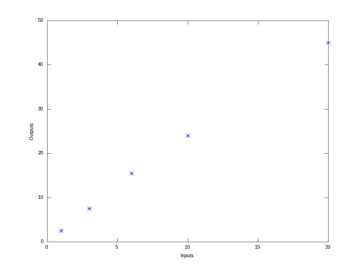
For the inputs of 1, 3, 6, 10, 20, we get the outputs as 2.5, 7.5, 15.5, 24, 45, respectively. Then, we would like to know as how is input is related to the output. So, to get a feel of the relation, we first plot this points on a x-y plane, say inputs as x and outputs as y. Figure 6 shows the same. And the octave code for that is as follows:

$ octave -qf
octave:1> x = [1 3 6 10 20];
octave:2> y = [2.5 7.5 15.5 24 45];
octave:3> plot(x, y, "*");
octave:4> xlabel("Inputs");
octave:5> ylabel("Outputs");
octave:6>
Figure 6: Plot of the data points

Figure 6: Plot of the data points

By observing the plot, the simplest fitting relation looks to be a straight line. So, let’s try fitting a linear polynomial, i.e. a first order polynomial, i.e. a straight line. Here’s the code in execution for it:

octave:1> x = [1 3 6 10 20];
octave:2> y = [2.5 7.5 15.5 24 45];
octave:3> p = polyfit(x, y, 1)
p =

   2.2212   1.1301

octave:4> polyout(p, "x");

2.2212*x^1 + 1.1301

octave:5> plot(x, y, "*", x, polyval(p, x), "-");
octave:6> xlabel("Inputs");
octave:7> ylabel("Outputs");
octave:8> legend("Data points", "Linear Fit");
octave:9>

polyfit() takes 3 arguments, the x values, the y values, and the order of the polynomial to fit – 1 for linear. It then returns the coefficients of the fitted polynomial p. polyout() displays the polynomial in more readable format. So, the fitted equation is y = 2.2212 * x + 1.1301. polyval() takes the polynomial p and the input values x, and calculates the output values y, as per the polynomial equation. And then we plot them, along with the earlier data points, on the same plot. Figure 7 shows the same, 2.2212 being the slope / gradient of the straight line, and 1.1301 being the intercept. Now, we notice that the straight line does not fit exactly, and there is some deviation from the observed points. polyfit() fits the polynomial with the minimum deviation for the order we request, but still there is a deviation, as that is the minimum possible. If you want to get the standard deviation for the particular fit, you just need to do the following:

octave:9> std_dev = sqrt(mean((y - polyval(p, x)).^2))
std_dev =  0.72637
octave:10>
Figure 7: Linear fit of data points

Figure 7: Linear fit of data points

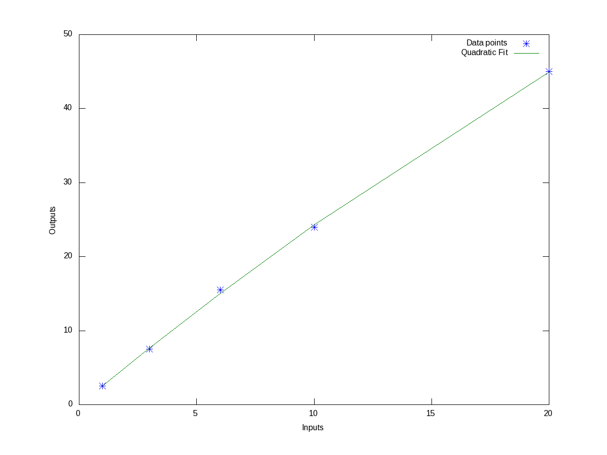
And we see that it is a small value compared to our output values. But say we are not fully satisfied with this, we may like to try higher order polynomials, say of order 2, a quadratic, and observe the results from it. Here’s how one would do this:

octave:1> x = [1 3 6 10 20];
octave:2> y = [2.5 7.5 15.5 24 45];
octave:3> p = polyfit(x, y, 2)
p =

  -0.018639   2.623382  -0.051663

octave:4> polyout(p, "x");

-0.018639*x^2 + 2.6234*x^1 - 0.051663

octave:5> plot(x, y, "*", x, polyval(p, x), "-");
octave:6> xlabel("Inputs");
octave:7> ylabel("Outputs");
octave:8> legend("Data points", "Quadratic Fit");
octave:9> std_dev = sqrt(mean((y - polyval(p, x)).^2))
std_dev =  0.26873
octave:10>

Figure 8 shows the data points and fitted quadratic curve. All the values above can be interpreted in the similar way as earlier. And we note that the standard deviation has come down further. In fact, as we increase the polynomial order further and further, we will definitely note that the standard deviation keeps on decreasing, till the order is same as number of data points – 1, after which it remains 0. But, we may not like to do this, as our observed data points are typically not perfect, and we are typically not interested in getting the standard deviation zero but for a fit more appropriate to reflect the relation between the system’s input and output.

Figure 8: Quadratic fit of data points

Figure 8: Quadratic fit of data points

Interpolation

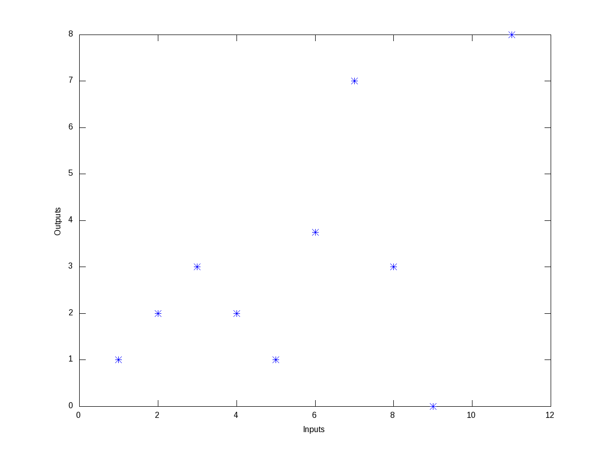
Now, say we have the following wierd data points, listed as (x, y) pairs: (1, 1), (2, 2), (3, 3), (4, 2), (5, 1), (6, 3.75), (7, 7), (8, 3), (9, 0), (11, 8). Figure 9 shows, how wierd they look like.

Figure 9: Wierd data points

Figure 9: Wierd data points

Trying to fit a polynomial, would be quite meaningless. But still they seem to have some correlation in between smaller ranges of input, say between 1 and 3, 3 and 5, 5 and 7, and so on. So, this is best suited for us to do interpolation for finding the values in between, say at 1.5, 3.8, 10, … Now interpolation is all about curve fitting between two neighbouring data points and then calculating the value at any intermediate point. So, the typical varieties of techniques used for this “piece-wise curve fitting” are:

  • nearest: Return the nearest data point (actually no curve fitting)
  • linear: Linear/Straight line fitting between the two neighbouring data points
  • pchip: Piece-wise cubic (order 3) hermite polynomial fitting
  • cubic: Cubic (order 3) polynomial fitted between four nearest neighbouring data points
  • spline: Cubic (order 3) spline fitting with smooth first and second derivatives throughout the curve

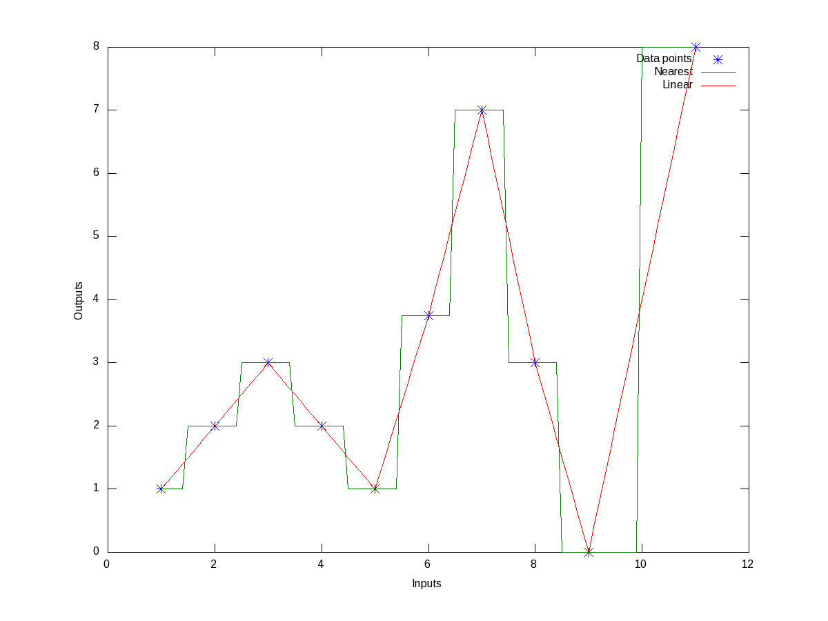
All these may look little jargonish – so don’t worry about that. Let’s just try out some examples to drive the point home. Here’s the code to show the nearest & linear interpolation for the above data:

octave:1> x = [1 2 3 4 5 6 7 8 9 11];
octave:2> y = [1 2 3 2 1 3.75 7 3 0 8];
octave:3> xi = 1:0.1:11;
octave:4> y_n = interp1(x, y, xi, "nearest");
octave:5> y_l = interp1(x, y, xi, "linear");
octave:6> plot(x, y, "*", xi, y_n, "-", xi, y_l, "-");
octave:7> xlabel("Inputs");
octave:8> ylabel("Outputs");
octave:9> legend("Data points", "Nearest", "Linear");
octave:10>

Figure 10 shows the same.

Figure 10: Nearest and linear interpolations of the data points

Figure 10: Nearest and linear interpolations of the data points

Now, if we want to get the interpolated values say at the points 1.5, 3.8, 10, instead of giving all the intermediate points xi in the above code, we may just give these 3 – that’s all. Here goes the code in execution for the that:

octave:1> x = [1 2 3 4 5 6 7 8 9 11];
octave:2> y = [1 2 3 2 1 3.75 7 3 0 8];
octave:3> our_x = [1.5 3.8 10];
octave:4> our_y_n = interp1(x, y, our_x, "nearest")
our_y_n =

   2   2   8

octave:5> our_y_l = interp1(x, y, our_x, "linear")
our_y_l =

   1.5000   2.2000   4.0000

octave:6>

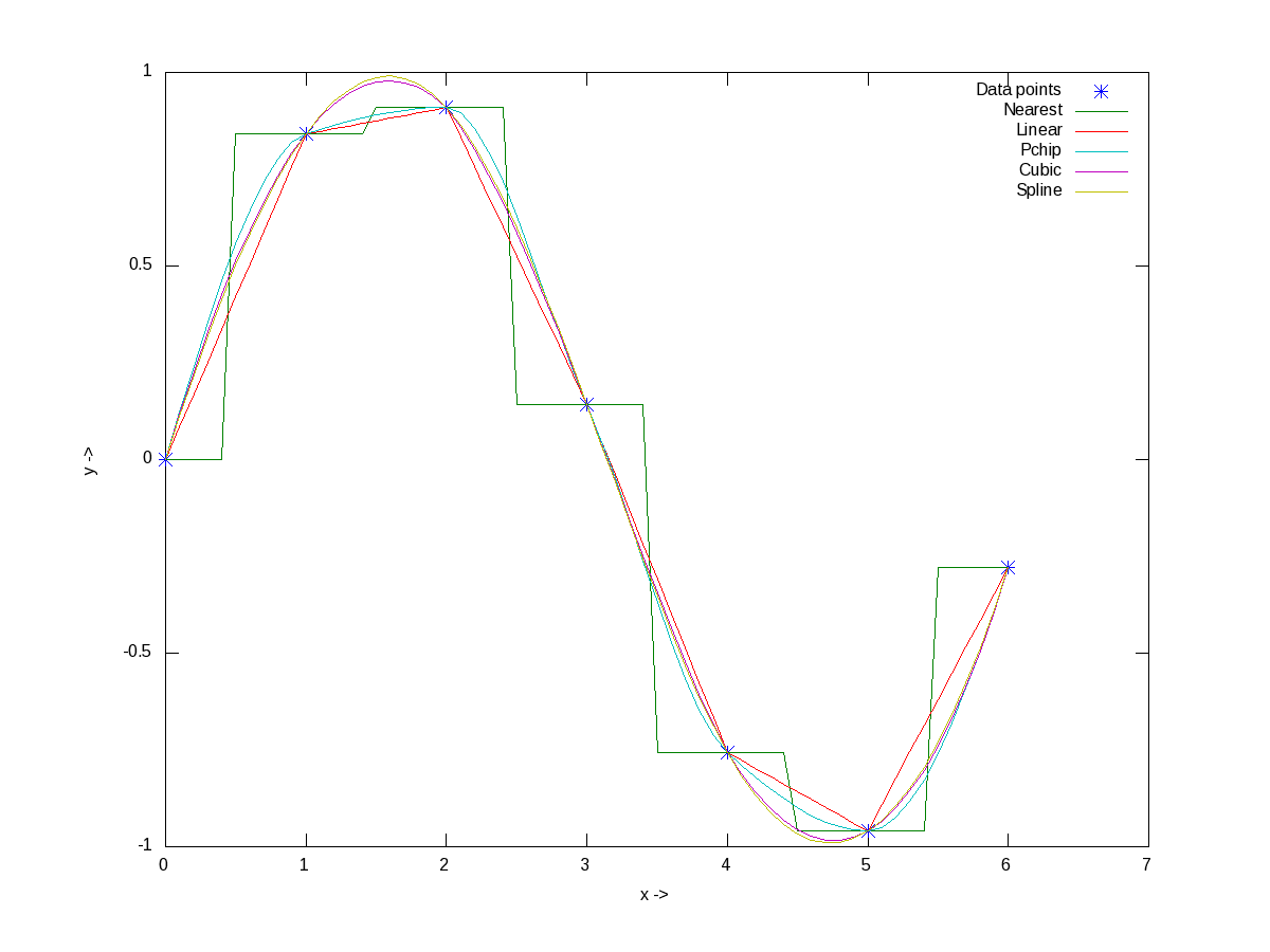
Now, before closing on interpolation, just to give a feel of all of the interpolation techniques, here goes an example with the points on a sine curve:

octave:1> x = 0:2*pi;
octave:2> y = sin(x);
octave:3> xi = 0:0.1:2*pi;
octave:4> y_n = interp1(x, y, xi, "nearest");
octave:5> y_l = interp1(x, y, xi, "linear");
octave:6> y_p = interp1(x, y, xi, "pchip");
octave:7> y_c = interp1(x, y, xi, "cubic");
octave:8> y_s = interp1(x, y, xi, "spline");
octave:9> plot(x, y, "*", xi, y_n, "-", xi, y_l, "-", xi, y_p, "-", xi, y_c, "-",
                                                                      xi, y_s, "-");
octave:10> xlabel("x ->");
octave:11> ylabel("y ->");
octave:12> legend("Data points", "Nearest", "Linear", "Pchip", "Cubic", "Spline");
octave:13> print("-dpng", "all_types_of_interpolations.png");
octave:14>

Figure 11 shows the visualization of the same for your eyes.

Figure 11: All types of interpolations for sinusoidal points

Figure 11: All types of interpolations for sinusoidal points

What’s next?

With today’s curve fitting & interpolation walk through, we have used some basic 2-D plotting techniques. But there are many more features and techniques to plotting, like marking our plots, visualizing 3-D stuff, etc. Next, we’ll look into that.

Twelfth Article >>

   Send article as PDF   

Kernel Space Debuggers in Linux

This tenth article, which is part of the series on Linux device drivers, talks about kernel space debugging in Linux.

<< Ninth Article

Shweta was back from hospital and relaxing in the library by reading up various books. Since the time she has known the ioctl way of debugging, she has been impatient to know more about debugging in kernel space. The basic curiosity coming from the fact that how and where would one run the kernel space debugger, if there is any. Contrast this with application/user space debugging, where we have the OS running underneath, and a shell or a GUI over it to run the debugger, say for example, the GNU debugger (gdb), the data display debugger (ddd). And viola, she came across this interesting kernel space debugging mechanism using kgdb, provided as part of the kernel itself, since kernel 2.6.26

Debugger challenge in kernel space

As we need some interface to be up, to run a debugger to debug anything, a debugger for debugging the kernel, could be visualized in 2 possible ways:

  1. Put the debugger into the kernel itself. And then the debugger runs from within, accessible through the usual monitor or console. An example of it is kdb. Until kernel 2.6.35, it was not official, meaning its source code was needed to be downloaded as 2 set of patches (one architecture dependent and one architecture independent) from ftp://oss.sgi.com/projects/kdb/download/ and then to be patched with the kernel source – though since kernel 2.6.35, majority of it is part of the kernel source’s official release. In either case, the kdb support needs to be enabled in the kernel source and then the kernel is to be compiled, installed and booted with. The boot screen itself would give the kdb debugging interface.
  2. Put a minimal debugging server into the kernel; a debugger client would then connect to it from a remote host system’s user space over some interface, say serial or ethernet. An example for that is kgdb – the kernel’s gdb server, to be used with gdb (client) from a remote system over either serial or ethernet. Since kernel 2.6.26, its serial interface part has been merged with kernel source’s official release. Though, if interested in its network interface part, it would still need to be patched with one of the releases from http://sourceforge.net/projects/kgdb/. In either case, the next step would be to enable kgdb support in the kernel source and then the kernel is to be compiled, installed and booted with – though this time to be connected with a remote debugger client.

Please note that in both the above cases, the complete kernel source for the kernel to be debugged is needed, unlike in case of building modules, where just headers are sufficient. Here is how to play around with kgdb over serial interface.

Setting up the Linux kernel with kgdb

Pre-requisite: Either kernel source package for the running kernel is installed on your system, or a corresponding kernel source release has been downloaded from http://kernel.org.

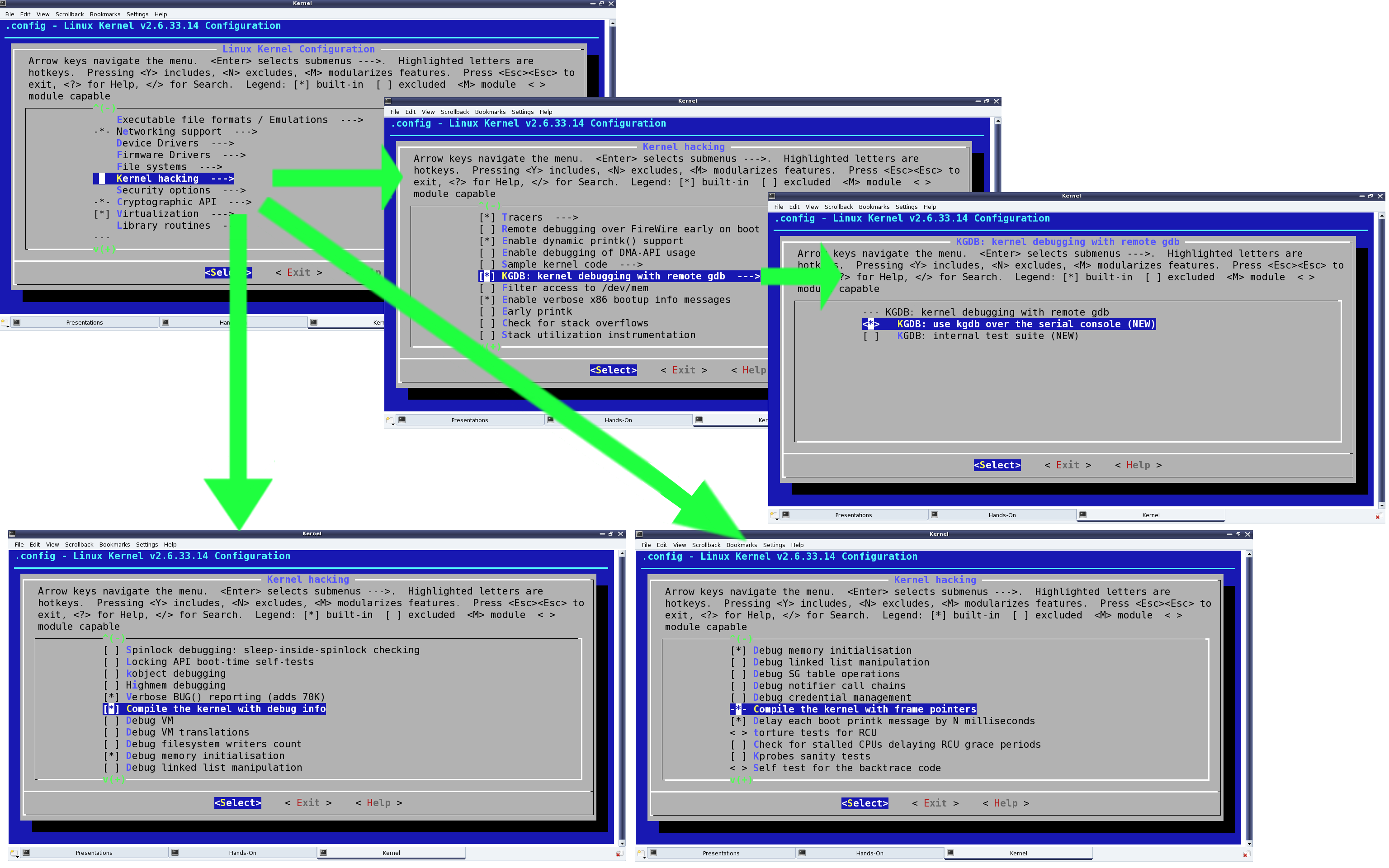
First of all, the kernel to be debugged need to have kgdb enabled and built into it. To achieve that, the kernel source has to be configured with CONFIG_KGDB=y. Additionally, for kgdb over serial, CONFIG_KGDB_SERIAL_CONSOLE=y needs to be configured. And CONFIG_DEBUG_INFO is preferred for symbolic data to be built into kernel for making debugging with gdb more meaningful. CONFIG_FRAME_POINTER=y enables frame pointers in the kernel allowing gdb to construct more accurate stack back traces. All these options are available under “Kernel hacking” in the menu obtained by issuing the following commands in the kernel source directory (preferably as root or using sudo):

$ make mrproper # To clean up properly
$ make oldconfig # Configure the kernel same as the current running one
$ make menuconfig # Start the ncurses based menu for further configuration

See the highlighted selections in Figure 15, for how and where would these options be:

  • “KGDB: kernel debugging with remote gdb” → CONFIG_KGDB
    • “KGDB: use kgdb over the serial console” → CONFIG_KGDB_SERIAL_CONSOLE
  • “Compile the kernel with debug info” → CONFIG_DEBUG_INFO
  • “Compile the kernel with frame pointers” → CONFIG_FRAME_POINTER
Figure 15: Configuring kernel with kgdb

Figure 15: Configuring kernel with kgdb

Once configured and saved, the kernel can be built by typing make in the kernel source directory. And then a make install is expected to install it, along with adding an entry for the installed kernel in the grub configuration file. Depending on the distribution, the grub configuration file may be /boot/grub/menu.lst, /etc/grub.cfg, or something similar. Once installed, the kgdb related kernel boot parameters, need to be added to this newly added entry.

Figure 16: grub configuration for kernel with kgdb

Figure 16: grub configuration for kernel with kgdb

Figure 16 highlights the kernel boot parameters added to the newly installed kernel, in the grub‘s configuration file.

kgdboc is for gdb connecting over console and the basic format is: kgdboc=<serial_device>,<baud_rate>
where:
<serial_device> is the serial device file on the system, which would run the kernel to be debugged, for the serial port to be used for debugging
<baud_rate> is the baud rate of the serial port to be used for debugging

kgdbwait enables the booting kernel to wait till a remote gdb (i.e. gdb on another system) connects to it, and this parameter should be passed only after kgdboc.

With this, the system is ready to reboot into this newly built and installed kernel. On reboot, at the grub‘s menu, select to boot from this new kernel, and then it will wait for gdb to connect with it from an another system over the serial port.

All the above snapshots have been with kernel source 2.6.33.14, downloaded from http://kernel.org. And the same should work for at the least any 2.6.3x release of kernel source. Also, the snapshots are captured for kgdb over serial device file /dev/ttyS0, i.e. the first serial port.

Setting up gdb on another system

Pre-requisite: Serial ports of the system to be debugged and the another system to run gdb from, should be connected using a null modem (i.e. a cross over serial) cable.

Here are the gdb commands to get the gdb from the other system connect to the waiting kernel. All these commands have to be given on the gdb prompt, after typing gdb on the shell.

Connecting over serial port /dev/ttyS0 (of the system running gdb) with baud rate 115200 bps:

$ gdb
...
(gdb) file vmlinux
(gdb) set remote interrupt-sequence Ctrl-C
(gdb) set remotebaud 115200
(gdb) target remote /dev/ttyS0
(gdb) continue

In the above commands, vmlinux is the kernel image built with kgdb enabled and needs to be copied into the directory on the system, from where gdb is being executed. Also, the serial device file and its baud rate has to be correctly given as per one’s system setup.

Debugging using gdb with kgdb

After this, it is all like debugging an application from gdb. One may stop execution using Ctrl+C, add break points using b[reak], step execution using s[tep] or n[ext], … – the usual gdb way. For details on how to use gdb, there are enough tutorials available online. In fact, if not comfortable with text-based gdb, the debugging could be made GUI-based, using any of the standard GUI tools over gdb, for example, ddd, Eclipse, etc.

Summing up

By now, Shweta was all excited to try out the kernel space debugging experiment using kgdb. And as she needed two systems to try it out, she decided to go to the Linux device drivers lab. There, she set up the system to be debugged, with the kgdb enabled kernel, and connected it with an another system using a null modem cable. Then on the second system, she executed gdb to remotely connect with and step through the kernel on the first system.

Eleventh Article >>

Notes

  1. Parameter for using kgdb over ethernet is kgdboe. It has the following format: kgdboe=[<this_udp_port>]@<this_ip>/[this_dev],[<remote_udp_port>]@<remote_ip>/[<remote_mac_addr>]

where:
<this_udp_port> is optional and defaults to 6443,
<this_ip> is IP address of the system, which would run the kernel to be debugged,
<this_dev> is optional and defaults to eth0,
<remote_udp_port> is optional and defaults to 6442,
<remote_ip> is IP address of the system, from which gdb would be connecting from,
<remote_mac_addr> is optional and defaults to broadcast.

Here are the gdb commands for connecting to kgdb over network port 6443 to IP address 192.168.1.2:

$ gdb
...
(gdb) file vmlinux
(gdb) set remotebreak 0
(gdb) target remote udp:192.168.1.2:6443
(gdb) continue
   Send article as PDF   

Polynomial Power of Octave

This tenth article of the mathematical journey through open source, explains advanced polynomial mathematics in octave.

<< Ninth Article

Roots of i

Let’s start with the solution to our previous brain teaser of finding the square and cube roots of the imaginary number i, which boils down to finding all the roots of the equations x2 = i and x3 = i, respectively. In other words, roots of the polynomials x2 – i and x3 – i, respectively, as follows:

$ octave -qf
octave:1> roots([1 0 -i])
ans =

   0.70711 + 0.70711i
  -0.70711 - 0.70711i

octave:2> roots([1 0 0 -i])
ans =

  -0.86603 + 0.50000i
  -0.00000 - 1.00000i
   0.86603 + 0.50000i

octave:3>

Displaying Polynomial

Before we start exploring polynomials further, here’s a couple of basic octave functions to visualize the polynomials. polyout() displays a polynomial in our usual known format. polyreduce() removes the redundant leading zero coefficients. Check out the following:

$ octave -qf
octave:1> p = [ 0 0 5 3 -9 4 6 ];
octave:2> polyout(p, "x");
0*x^6 + 0*x^5 + 5*x^4 + 3*x^3 - 9*x^2 + 4*x^1 + 6
octave:3> polyreduce(p)
ans =

   5   3  -9   4   6

octave:4> polyout(polyreduce(p), "x");
5*x^4 + 3*x^3 - 9*x^2 + 4*x^1 + 6
octave:5>

Polynomial Arithmetic

As octave represents polynomial as vectors, their addition and subtraction are vector addition and subtraction, respectively. However, the polynomial vectors may be of different length. Hence, they need to be made of same length before addition or subtraction. So, let’s write functions to do the complete operations:

function [ q1 q2 ] = equalize(p1, p2)
# Assuming p1 & p2 to be row vectors
    m = max(length(p1), length(p2));
    q1 = [ zeros(1, m - length(p1)) p1 ];
    q2 = [ zeros(1, m - length(p2)) p2 ];
endfunction

function p = polyadd(p1, p2)
    [ q1 q2 ] = equalize(p1, p2);
    p = polyreduce(q1 + q2);
endfunction

function p = polysub(p1, p2)
    [ q1 q2 ] = equalize(p1, p2);
    p = polyreduce(q1 - q2);
endfunction

Assuming the above code is put in the file polynomials.oct, the same can be used as follows:

$ octave -qf
octave:1> source("polynomials.oct");
octave:2> polyout(p1 = [ 1 2 1 ], "x");
1*x^2 + 2*x^1 + 1
octave:3> polyout(p2 = [ 1 -1 ], "x");
1*x^1 - 1
octave:4> polyout(polyadd(p1, p2), "x");
1*x^2 + 3*x^1 + 0
octave:5> polyout(polysub(p1, p2), "x");
1*x^2 + 1*x^1 + 2
octave:6>

Interestingly, octave already have the functions for multiplication and division of polynomials, namely conv() and deconv(), respectively. Here’s a demonstration:

$ octave -qf
octave:1> polyout(p1 = [ 1 2 1 ], "x");
1*x^2 + 2*x^1 + 1
octave:2> polyout(p2 = [ 1 -1 ], "x");
1*x^1 - 1
octave:3> polyout(conv(p1, p2), "x");
1*x^3 + 1*x^2 - 1*x^1 - 1
octave:4> polyout(deconv(p1, p2), "x");
1*x^1 + 3
octave:5> [ q r ] = deconv(p1, p2)
q =

   1   3

r =

   0   0   4

octave:6>

Polynomial Differentiation and Integration

Octave also provides functions for differentiation and integration of polynomials, namely polyder() and polyint(). Here goes an example of differentiation and definite integral using the same:

$ octave -qf
octave:1> polyout(p = [ 1 2 1 ], "x");
1*x^2 + 2*x^1 + 1
octave:2> polyout(polyder(p), "x");
2*x^1 + 2
octave:3> polyout(polyint(p), "x");
0.33333*x^3 + 1*x^2 + 1*x^1 + 0
octave:4> q = polyint(p);
octave:5> polyval(q, 3) - polyval(q, 0) # Definite integral of p from 0 to 3
ans =  21
octave:6>

What’s next?

Given a set of data points a common requirement in fields of physics, statistics, and many others is to fit a polynomial to it. Going further, we’ll explore the power of octave for the same.

Eleventh Article >>

   Send article as PDF