Tag Archives: Maths

Doing Algebra with Maxima

This fourteenth article of the mathematical journey through open source, introduces to doing algebra using Maxima.

<< Thirteenth Article

Maxima is a computer algebra system derived from the earlier Macsyma, which in turn, was written in Lisp.

Algebraic capability of Maxima is the one, which puts it apart from the others. We have worked through basic shell maths, bench calculator bc, and finally the ultra capable octave. But none of them could do algebra with symbols, also referred as symbolic or analytic mathematics. Let’s walk through a few examples to demonstrate what it means.

Getting started

Maxima command line can be started on the shell by typing maxima. -q option to it suppresses the initial welcome message. Typing quit(); on the Maxima command line quits Maxima. Typical Maxima commands shall be terminated either with a semicolon (;) or a dollar ($) – the later suppressing any print from the command. Outputs are numbered and prefaced by %o. Inputs are also numbered, and prefaced by %i. Here are a few factorization examples:

$ maxima -q
(%i1) factor(x^3 - 1);
                                       2
(%o1)                        (x - 1) (x  + x + 1)
(%i2) factor((x + 1)^4);
                                     4
(%o2)                              (x + 1)
(%i3) expand(%o2);
                           4      3      2
(%o3)                     x  + 4 x  + 6 x  + 4 x + 1
(%i4) factor(6!);
                                     4  2
(%o4)                               2  3  5
(%i5) expand(6!);
(%o5)                                 720
(%i6) quit();

factor() and expand() are two complementary functions doing factorization & simplification, respectively. Note the way the powers in the output are printed. For example, 6! is factorized as 24 * 32 * 5. In case, we want the output on a single line, we may use the command string(), which we shall use now onwards. Also, note the usage of output labels as inputs to the commands, namely expand(%o2) in the above example.

Integration and differentiation

Octave has enabled us to do integration and differentiation, but more of definite integrals and differences. Yes, it has indefinite operations for polynomials. But with Maxima, we can just plug in the expressions, as we usually do on our maths notebooks. This is what it means:

$ maxima -q
(%i1) integrate(cos(x),x);
(%o1)                               sin(x)
(%i2) diff(cos(x),x);
(%o2)                              - sin(x)
(%i3) string(integrate(1/(a^2 + x^2)^(3/2),x));
(%o3)                        x/(a^2*sqrt(x^2+a^2))
(%i4) string(diff(log(x), x));
(%o4)                                 1/x
(%i5) y: (x+1)^2$ /* $ suppresses the output */
(%i6) string(diff(y, x));
(%o6)                              2*(x+1)
(%i7) string(integrate(y, x));
(%o7)                            x^3/3+x^2+x
(%i8) quit();

Variable assignments can be done in Maxima using colon (:), as shown in the input %i5, above. There onwards, the variable can be used instead of the original expression, as shown in the inputs %i6 & %i7. Note that the variable assignment assigns the complete symbolic expression, unlike the usual value assignments.

Solving equations

Whether it be linear set of equations, polynomial equations, or for that matter non-linear equations, Maxima can solve most of them with quite ease, and that also in a analytical way. Here are a few common examples: 1) The two solutions of a quadratic equation; 2) Two simultaneous equations in two variables; 3) A non-linear equation with irrational number e. Maxima code demonstration follows:

$ maxima -q
(%i1) string(solve(a*x^2 + b*x + c = 0, x));
(%o1)   [x = -(sqrt(b^2-4*a*c)+b)/(2*a),x = (sqrt(b^2-4*a*c)-b)/(2*a)]
(%i2) string(solve([a*x + b*y = c,d*x + e*y = f],[x, y]));
(%o2)        [[x = -(c*e-b*f)/(b*d-a*e),y = (c*d-a*f)/(b*d-a*e)]]
(%i3) string(solve([exp(x) + 1/exp(x) = a],[x]));
(%o3)      [x = log(a/2-sqrt(a^2-4)/2),x = log(sqrt(a^2-4)/2+a/2)]
(%i8) quit();

Equation solving has been one of the most fascinating as well as challenging tasks for solving mathematical problems, since ages. So, when the computer is there to aid it, we try to go beyond the human limitations. We just saw the well-known formula for the two solutions of a quadratic equation. How about the same for a cubic equation? It looks really complicated and hence we typically don’t use it. But, still you want to see it. Here it goes:

$ maxima -q
(%i1) string(solve(a*x^3 + b*x^2 + c*x + d = 0, x));
(%o1) [x = (-sqrt(3)*%i/2-1/2)*(sqrt(27*a^2*d^2+(4*b^3-18*a*b*c)*d+4*a*c^3-b^2*c^2)/
(2*3^(3/2)*a^2)-(27*a^2*d-9*a*b*c+2*b^3)/(54*a^3))^(1/3)-(sqrt(3)*%i/2-1/2)*(3*a*c-
b^2)/(9*a^2*(sqrt(27*a^2*d^2+(4*b^3-18*a*b*c)*d+4*a*c^3-b^2*c^2)/(2*3^(3/2)*a^2)-
(27*a^2*d-9*a*b*c+2*b^3)/(54*a^3))^(1/3))-b/(3*a),x = (sqrt(3)*%i/2-1/2)*(sqrt(27*
a^2*d^2+(4*b^3-18*a*b*c)*d+4*a*c^3-b^2*c^2)/(2*3^(3/2)*a^2)-(27*a^2*d-9*a*b*c+2*b^3)/
(54*a^3))^(1/3)-(-sqrt(3)*%i/2-1/2)*(3*a*c-b^2)/(9*a^2*(sqrt(27*a^2*d^2+(4*b^3-18*a*
b*c)*d+4*a*c^3-b^2*c^2)/(2*3^(3/2)*a^2)-(27*a^2*d-9*a*b*c+2*b^3)/(54*a^3))^(1/3))-b/
(3*a),x = (sqrt(27*a^2*d^2+(4*b^3-18*a*b*c)*d+4*a*c^3-b^2*c^2)/(2*3^(3/2)*a^2)-(27*
a^2*d-9*a*b*c+2*b^3)/(54*a^3))^(1/3)-(3*a*c-b^2)/(9*a^2*(sqrt(27*a^2*d^2+(4*b^3-18*
a*b*c)*d+4*a*c^3-b^2*c^2)/(2*3^(3/2)*a^2)-(27*a^2*d-9*a*b*c+2*b^3)/(54*a^3))^(1/3))-
b/(3*a)]
(%i2) quit();

And that’s what is the power of Maxima.

Plotting graphs

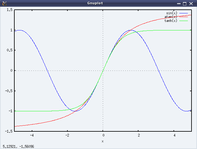
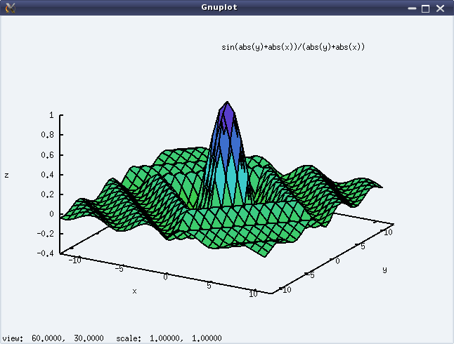
Along with the algebraic processing, Maxima also supports graph plotting for the algebraic expressions, though we must specify the intervals to plot it. It can do 2-D as well as 3-D plots. The following code shows an example for each of these. And figures 22 & 23 show the respective plots.

$ maxima -q
(%i1) plot2d([sin(x), atan(x), tanh(x)], [x, -5, 5])$
(%i2) plot3d(sin(abs(x) + abs(y))/(abs(x) + abs(y)),[x, -12, 12], [y, -12, 12])$
(%i3) quit();
Figure 22: Output of plot2d()

Figure 22: Output of plot2d()

Figure 23: Output of plot3d()

Figure 23: Output of plot3d()

After this first glimpse of what Maxima can do, we are now ready to move on to detail out the specific topics, like expression simplification, polynomials, etc.
Fifteenth Article >>

   Send article as PDF   

Octavian Statistics

This thirteenth article of the mathematical journey through open source, gives a glimpse of statistical capabilities of octave.

<< Twelfth Article

Statistics – the name itself brings to the mind the thought of data, and the associated probabilities, averages, deviations, random numbers. Rather than getting perplexed by all these, octave shows out how to use them in a very conducive way.

Data moments

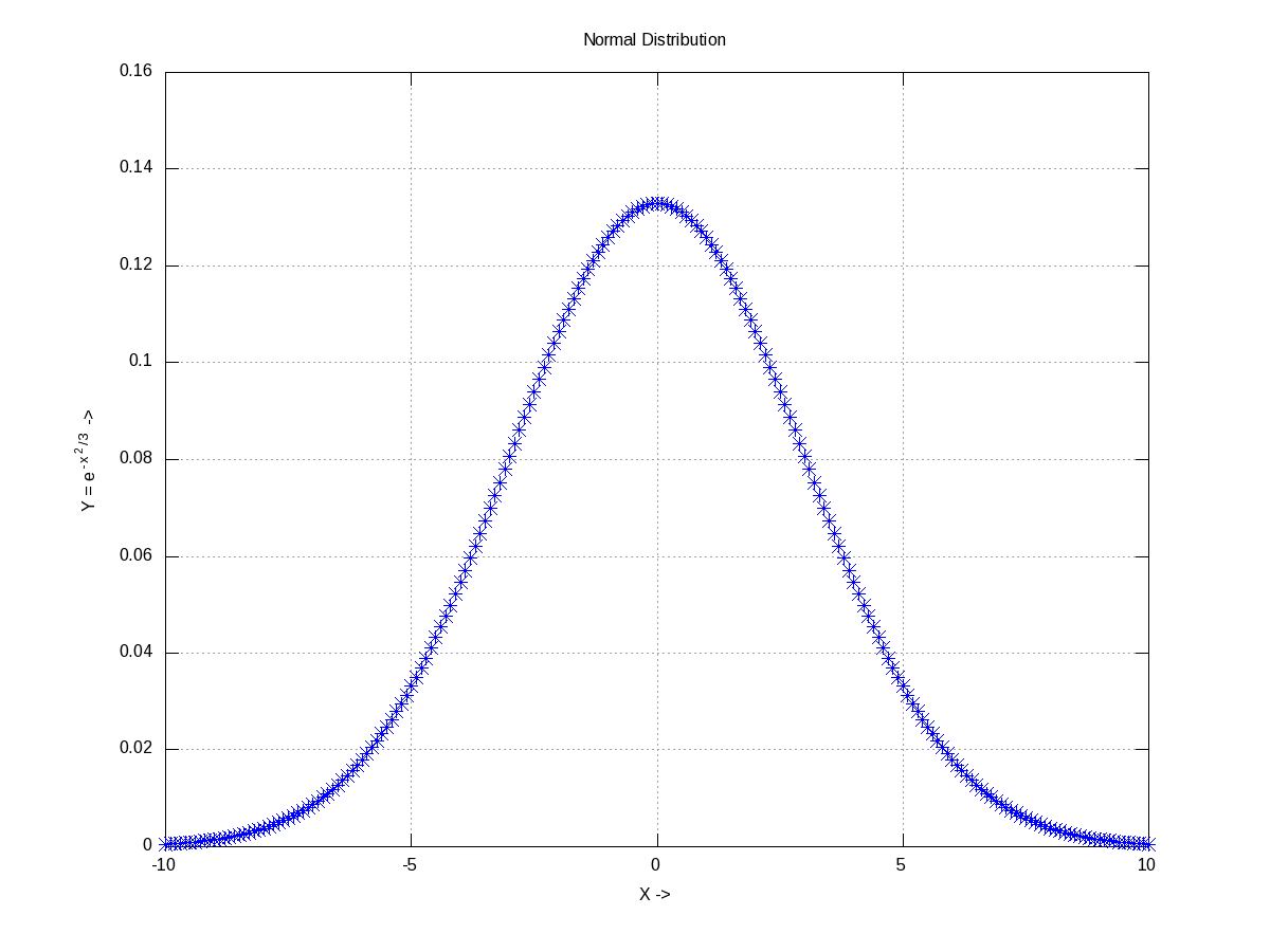
Already got scared by the name itself. Don’t worry. Moments basically mean the various kinds of averages, median, modes, etc. To understand them, let’s take some random data set, which may be generated using any of the various distributions. Let’s take the most “natural” normal distribution – yes the bell-shaped one. Figure 19 shows one centered around 0 (the mean) with a spread of 3 (the standard deviation), generated using normpdf(), as cited below. Note that octave has a whole set of all such functions.

$ octave -qf
octave:1> X = -10:0.1:10;
octave:2> Y = normpdf(X, 0, 3); # Normal Density Function
octave:3> plot(X, Y, "b*");
octave:4> xlabel("X ->");
octave:5> ylabel("Y = e^{-{x^2}/3} ->");
octave:6> title("Normal Distribution");
octave:7> grid("on");
octave:8>
Figure 19: Normal distribution with mean = 0, std = 3

Figure 19: Normal distribution with mean = 0, std = 3

If we take all the infinite points on this curve, would get a mean of 0 and a standard deviation of 3. But that’s not practical. So, let’s pick, say 10 random points from it. normrnd(m, s, 10, 1) provides the same in a 10×1 vector, following the normal distribution of mean m & standard deviation s. And then, mean() & std() give the mean and standard deviation, respectively. mean() could be of three types: Ordinary (arithmetic) mean (“a”), Geometric mean (“g”), Harmonic mean (“h”).

$ octave -qf
octave:1> Y = normrnd(0, 3, 10, 1) # m=0; s=3; 10x1 vector
Y =

  -2.33218
  -3.16866
   3.41991
  -2.27566
  -1.45403
   7.79691
   2.12849
   2.32727
  -5.37920
  -0.63447
octave:2> mean(Y)
ans =  0.042839
octave:3> mean(Y, "h")
ans =  -4.3226
octave:4> std(Y)
ans =  3.8662
octave:5> median(Y)
ans = -1.0442
octave:6> cov(Y, Y)
ans =  14.947
octave:7> cor(Y, Y)
ans =  1
octave:8>

Among many other moments, the four common ones are: 1) median() gets the middle most element in the sorted arrangement of data; 2) mode() gets the most frequently occurring data point; 3) cov() gives the variance between two set of data points, i.e. the covariance; 4) cor() gives the relation between two set of data points, i.e. the correlation ranging from -1 to 1. Correlation of 1 indicating they are completely related, 0 indicating totally unrelated, and a -1 indicating related completely but in an opposite sense.

Visualizing the probabilities

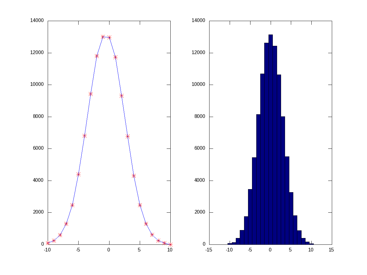
Random numbers are a beautiful example of probabilities. They occur as per their probabilities decided by the probability density function (PDF) they follow. Let’s visualize that using a live example. So again, as in the above example, let’s take some random numbers following the normal distribution. But, this time we’ll take a lot more points, say 1,00,000 points, so that we can actually see them following the bell-shape. But still, we are not having infinite points to give the continuous bell. So, what we have to do is collect the random points around some pre-designated buckets of fixed ranges. That is what we call a histogram. histc() does exactly that, returning the number of points in each of the buckets, which we can then plot to see our bell. Another function hist(), does all those in a more beautiful way. Figure 20 shows the two plots, for which the code follows:

$ octave -qf
octave:1> Y=normrnd(0, 3, 100000, 1); # 1 lakh random points
octave:2> B=-10:1:10; # Bucket edges -10, -9, ..., 10, i.e. 21 buckets
octave:3> N=histc(Y, B);
octave:4> subplot(1, 2, 1);
octave:5> plot(B, N, "r*", B, N, "b-");
octave:6> subplot(1, 2, 2);
octave:7> hist(Y, B); # More beautiful boxy plot
octave:8>
Figure 20: Histograms of normal distributed random points

Figure 20: Histograms of normal distributed random points

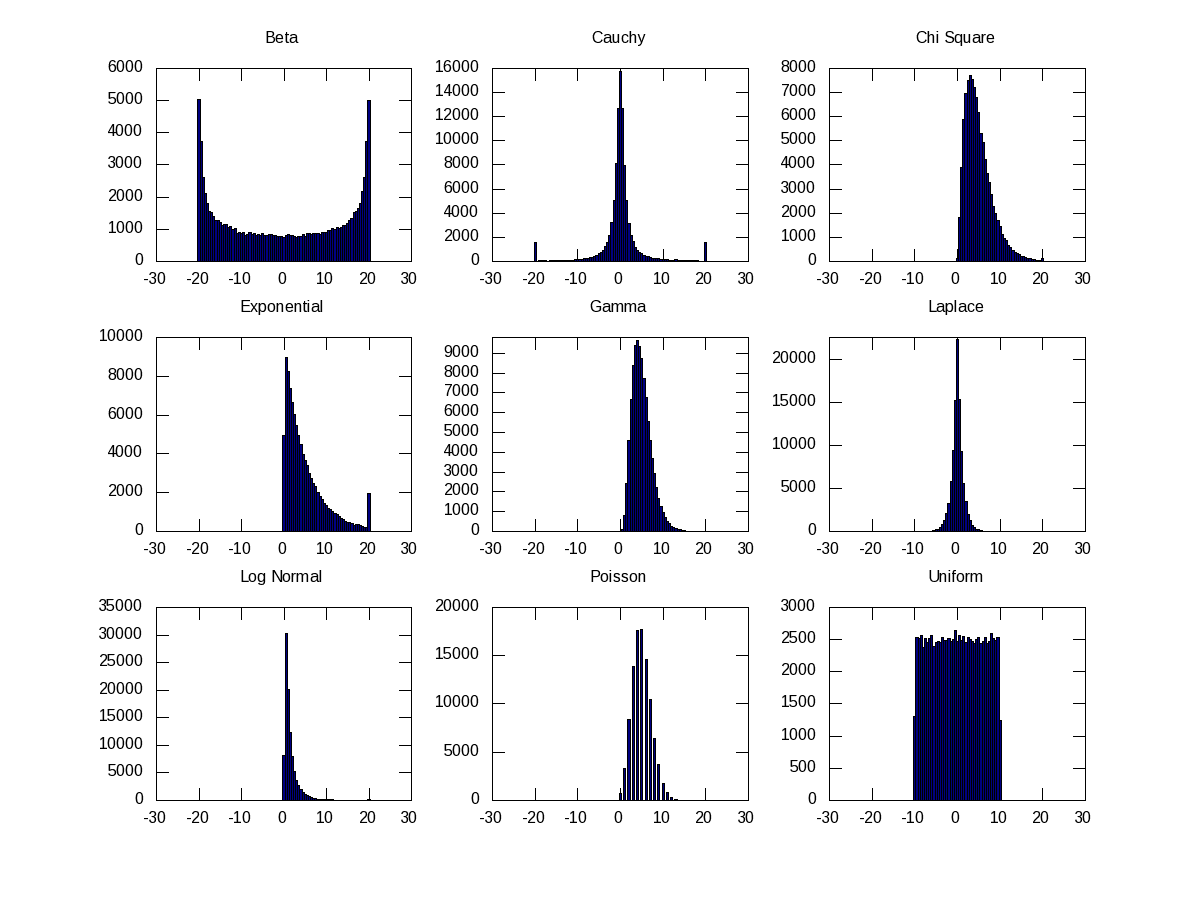
Similarly, if we use other PDFs, we would see similar histograms for them as well. Figure 21 shows nine such others, namely Beta (with alpha = beta = 0.5), Cauchy, Chi-Square, Exponential, Gamma, Laplace, Log Normal, Poisson, Uniform, using their respective functions, as shown in the code below:

octave:1> B=-20:0.5:20;
octave:2> subplot(3, 3, 1);
octave:3> hist(40*(betarnd(0.5, 0.5, 100000, 1) - 0.5), B);
octave:4> title("Beta");
octave:5> subplot(3, 3, 2);
octave:6> hist(cauchy_rnd(0, 1, 100000, 1), B);
octave:7> title("Cauchy");
octave:8> subplot(3, 3, 3);
octave:9> hist(chi2rnd(5, 100000, 1), B);
octave:10> title("Chi Square");
octave:11> subplot(3, 3, 4);
octave:12> hist(exprnd(5, 100000, 1), B);
octave:13> title("Exponential");
octave:14> subplot(3, 3, 5);
octave:15> hist(gamrnd(5, 1, 100000, 1), B);
octave:16> title("Gamma");
octave:17> subplot(3, 3, 6);
octave:18> hist(laplace_rnd(100000, 1), B);
octave:19> title("Laplace");
octave:20> subplot(3, 3, 7);
octave:21> hist(lognrnd(0, 1, 100000, 1), B);
octave:22> title("Log Normal");
octave:23> subplot(3, 3, 8);
octave:24> hist(poissrnd(5, 100000, 1), B);
octave:25> title("Poisson");
octave:26> subplot(3, 3, 9);
octave:27> hist(unifrnd(-10, 10, 100000, 1), B);
octave:28> title("Uniform");
octave:29>
Figure 21: Histograms of probability density functions

Figure 21: Histograms of probability density functions

Miscellaneous helpers

Apart from the standard ones, discussed so far, there are quite a few miscellaneous useful functions provided by octave. Here are a few:

  • perms() – Generates the n! permutations of the data points
  • values() – Sorts the data into non-repeating ascending order
  • range() – Returns the difference between the maximum and the minimum data points

Here follows a demonstration:

$ octave -qf
octave:1> perms([0 1 2])
ans =

   0   1   2
   1   0   2
   0   2   1
   1   2   0
   2   0   1
   2   1   0

octave:2> values([1 4 -9 -7 0 -6 12 -90])
ans =

  -90
   -9
   -7
   -6
    0
    1
    4
   12

octave:3> range([1 4 -9 -7 0 -6 12 -90])
ans =  102
octave:4>

What’s next?

Till date, in all our mathematical explorations, we have been always dealing with numbers. Ya! So big deal – anyways mathematics is about numbers, only. Not really. Many a times, we come across scenarios, where we would like to solve something symbolically or analytically, and then use numbers only at the end. Such things would not be possible with any of the OSS tools, we have discussed till now. But, yes there are such tools. One such is Maxima. And that’s where we are headed to next.

Fourteenth Article >>

   Send article as PDF   

Figures, Graphs, and Plots in Octave

This twelfth article of the mathematical journey through open source, shows the mathematical visualization in octave.

<< Eleventh Article

Mathematics is incomplete without visualization, without drawing the results, and without plotting the graphs. octave uses the powerful gnuplot as the backend of its plotting functionality. And in the frontend provides various plotting functions. Let’s look at the most beautiful ones.

Basic 2D Plotting

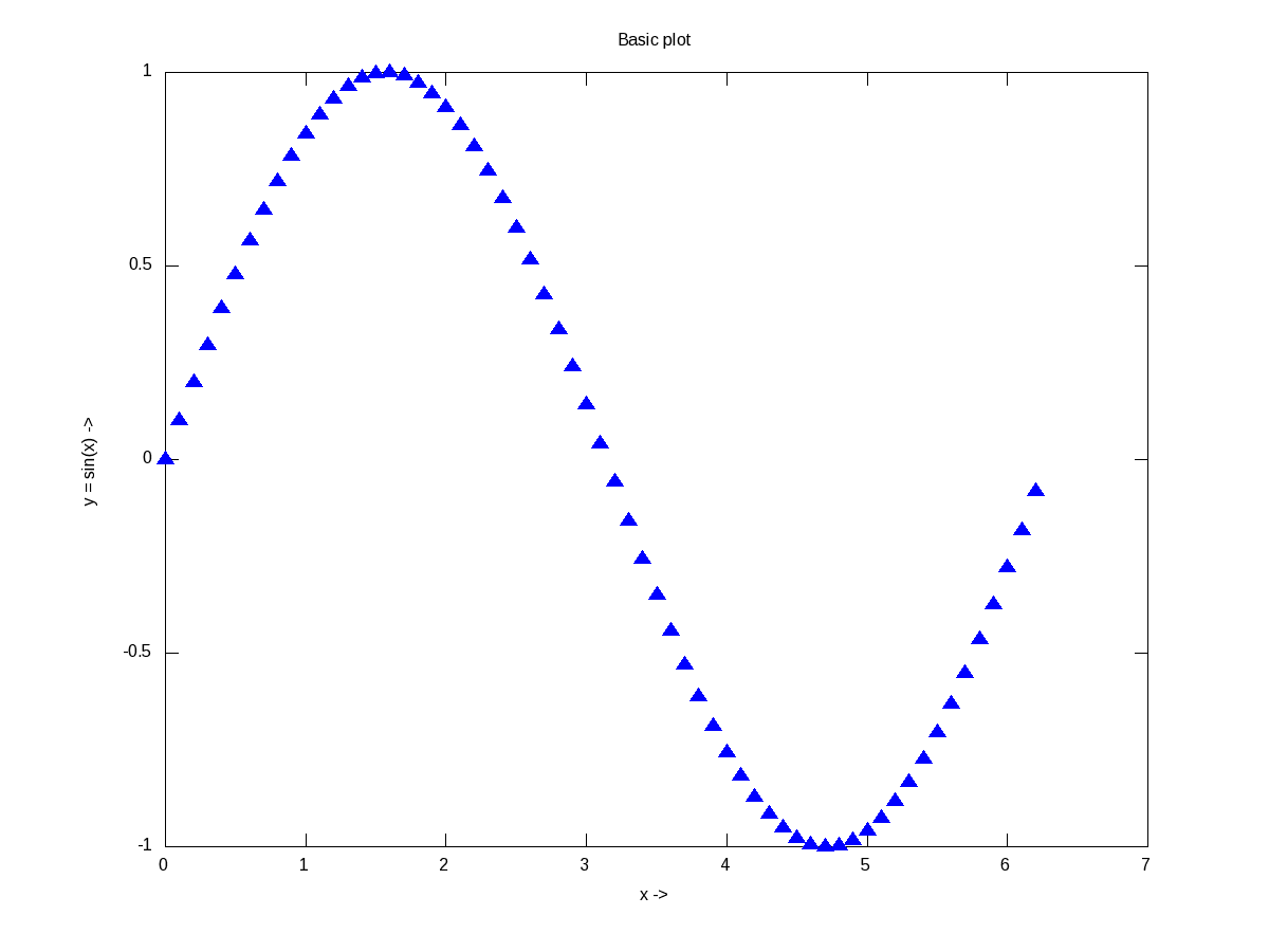
The most basic plotting is using the plot() function, which takes the Cartesian x & y values. Additionally, you may pass, as how to plot, i.e. as points or lines, their style, their colour, label, etc. Supported point styles are: +, *, o, x, ^, and lines are represented by -. Supported colours are: k (black), r (red), g (green), b (blue), y (yellow), m (magenta), c (cyan), w (white). With this background, here is how you plot a sine curve, and Figure 12 shows the plot.

$ octave -qf
octave:1> x = 0:0.1:2*pi;
octave:2> y = sin(x);
octave:3> plot(x, y, "^b");
octave:4> xlabel("x ->");
octave:5> ylabel("y = sin(x) ->");
octave:6> title("Basic plot");
octave:7>
Figure 12: Basic plotting in octave

Figure 12: Basic plotting in octave

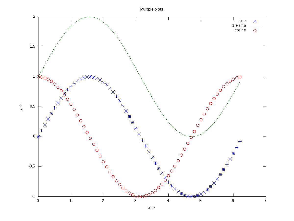
xlabel(), and ylabel() adds the corresponding labels, and title() adds the title. Multiple plots can be done on the same axis as follows, and Figure 13 shows the plots. Note the usage of legend() to mark the multiple plots.

$ octave -qf
octave:1> x = 0:0.1:2*pi;
octave:2> plot(x, sin(x), "*", x, 1 + sin(x), "-", x, cos(x), "o");
octave:3> xlabel("x ->");
octave:4> ylabel("y ->");
octave:5> legend("sine", "1 + sine", "cosine");
octave:6> title("Multiple plots");
octave:7>
Figure 13: Multiple plots on the same axis

Figure 13: Multiple plots on the same axis

Advanced 2D Figures

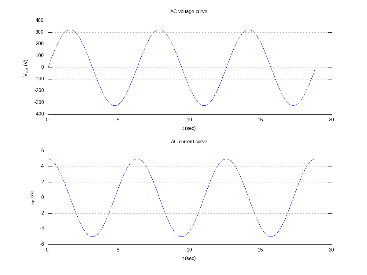
Now, if we want to have the multiple graphs on the same sheet but with different axes as shown in Figure 14, here is how to do that:

octave:1> t = 0:0.1:6*pi;
octave:2> subplot(2, 1, 1);
octave:3> plot(t, 325 * sin(t));
octave:4> xlabel("t (sec)");
octave:5> ylabel("V_{ac} (V)");
octave:6> title("AC voltage curve");
octave:7> grid("on");
octave:8> subplot(2, 1, 2);
octave:9> plot(t, 5 * cos(t));
octave:10> xlabel("t (sec)");
octave:11> ylabel("I_{ac} (A)");
octave:12> title("AC current curve");
octave:13> grid("on");
octave:14> print("-dpng", "multiple_plots_on_a_sheet.png");
octave:15>
Figure 14: Multiple plots on a sheet

Figure 14: Multiple plots on a sheet

Note the usage of subplot(), taking the matrix dimensions (row, column) and the plot number to create the matrix of plots. In the example above, it created a 2×1 matrix of plots. As add-ons, we have used the grid(“on”) to show up the dotted grid lines, and print() to save the generated figure as a .png file.

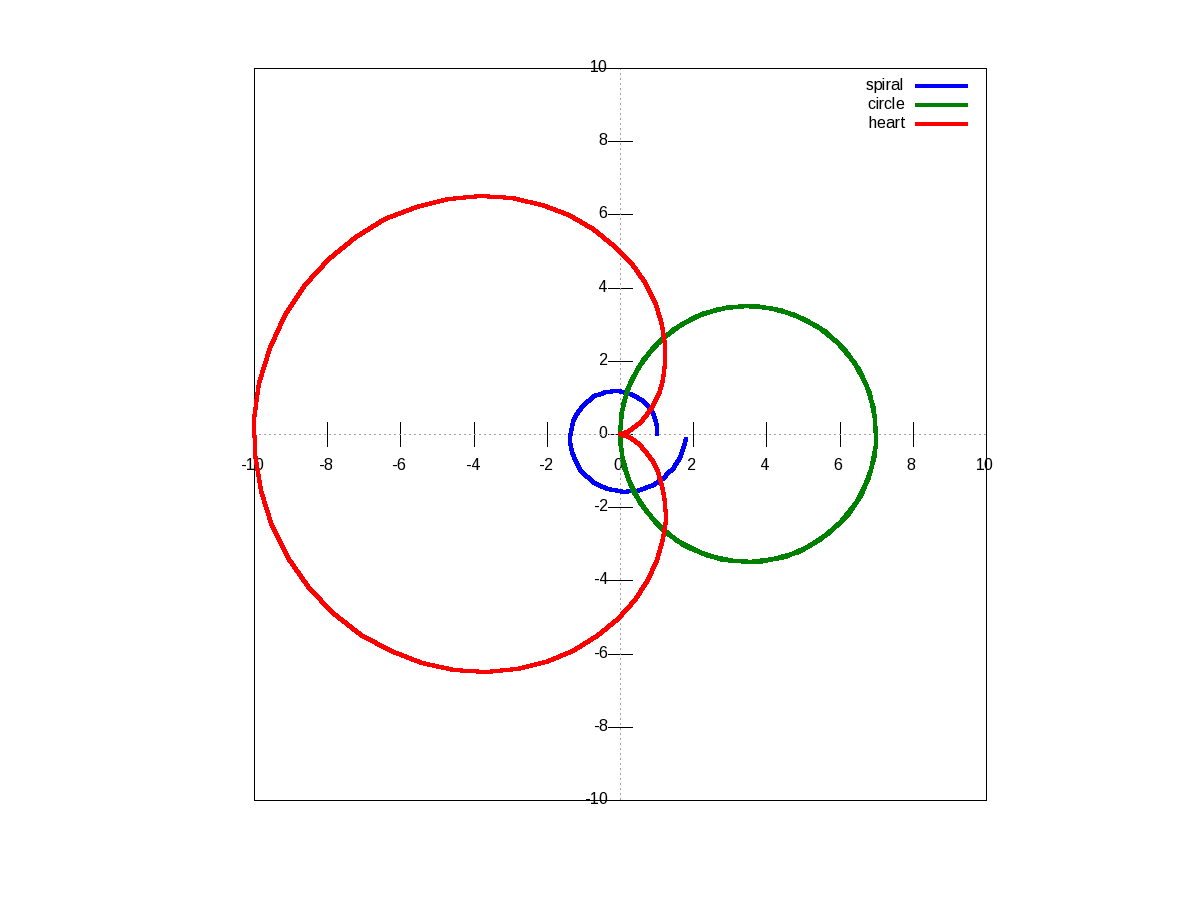
It is not always easy to plot everything in Cartesian co-ordinates, or rather many things are easier to plot in polar co-ordinates, e.g. a spiral, circle, heart, etc. The following code & Figure 15 shows a few such examples. Shown along with is a technique of modifying the figure properties, after drawing the figure using the set() function. Here it modifies the line thickness.

octave:1> th = 0:0.1:2*pi;
octave:2> r1 = 1.1 .^ th;
octave:3> r2 = 7 * cos(th);
octave:4> r3 = 5 * (1 - cos(th));
octave:5> r = [r1; r2; r3];
octave:6> ph = polar(th, r, "-");
octave:7> set(ph, "LineWidth", 4);
octave:8> legend("spiral", "circle", "heart");
octave:9>
Figure 15: Polar plots

Figure 15: Polar plots

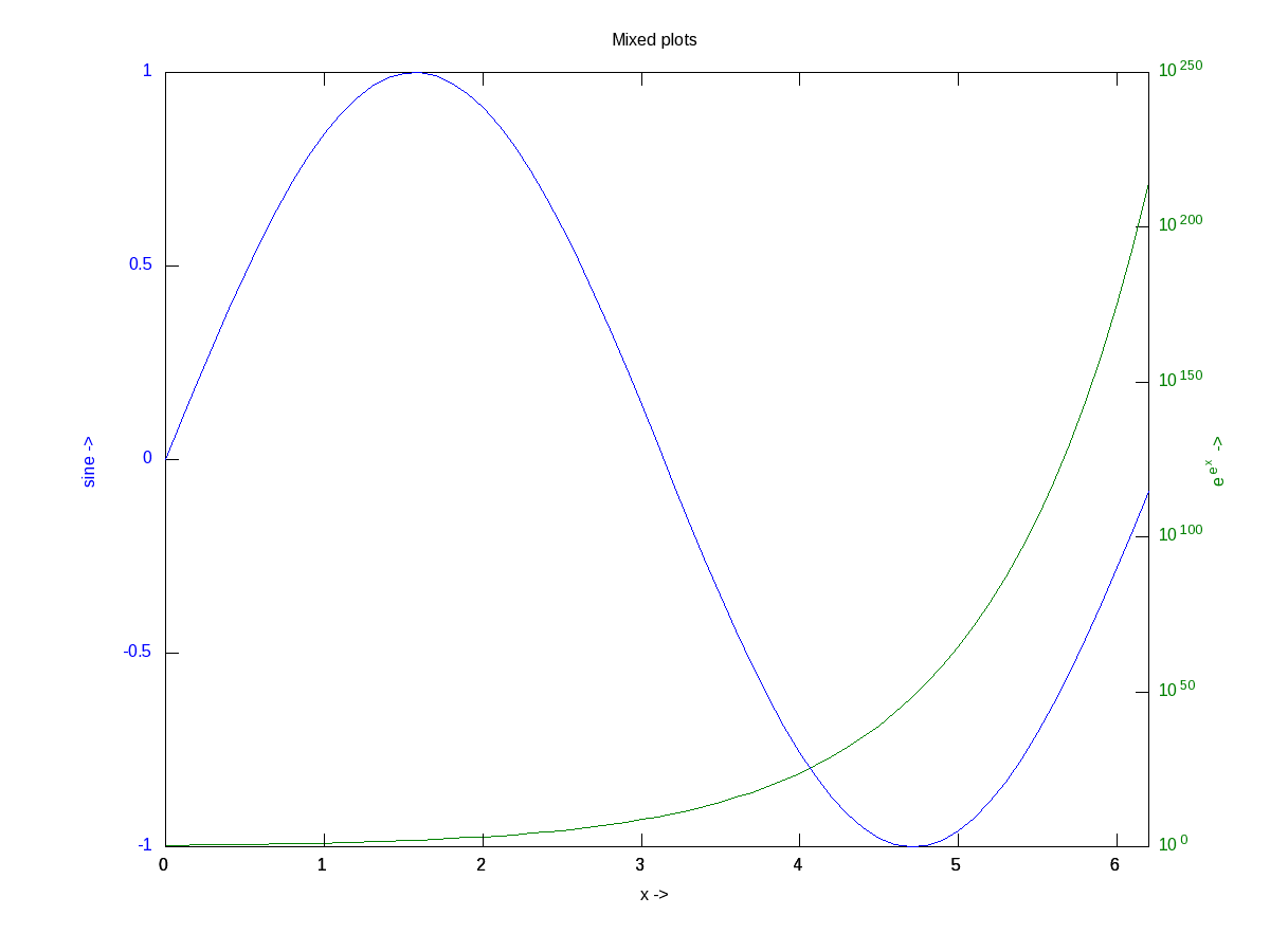
There are many other possible ways of drawing various interesting 2-D figures for all kind of mathematical & scientific requirements. So, before closing on 2-D plotting, let’s look into just one more often needed drawing – plotting with log axis, and more over with two y-axes on a single plot. The function for that is plotyy(). Note the plotyy() calling the corresponding function pointers @plot, @semilogy passed to it, in the following code segment. Figure 16 shows the output.

octave:1> x = 0:0.1:2*pi;
octave:2> y1 = sin(x);
octave:3> y2 = exp(exp(x));
octave:4> ax = plotyy(x, y1, x, y2, @plot, @semilogy);
octave:5> xlabel("x ->");
octave:6> ylabel(ax(1), "sine ->");
octave:7> ylabel(ax(2), "e^{e^x} ->");
octave:8> title("Mixed plots");
octave:9>
Figure 16: Mixed plots with semi log axis

Figure 16: Mixed plots with semi log axis

3D Visualization

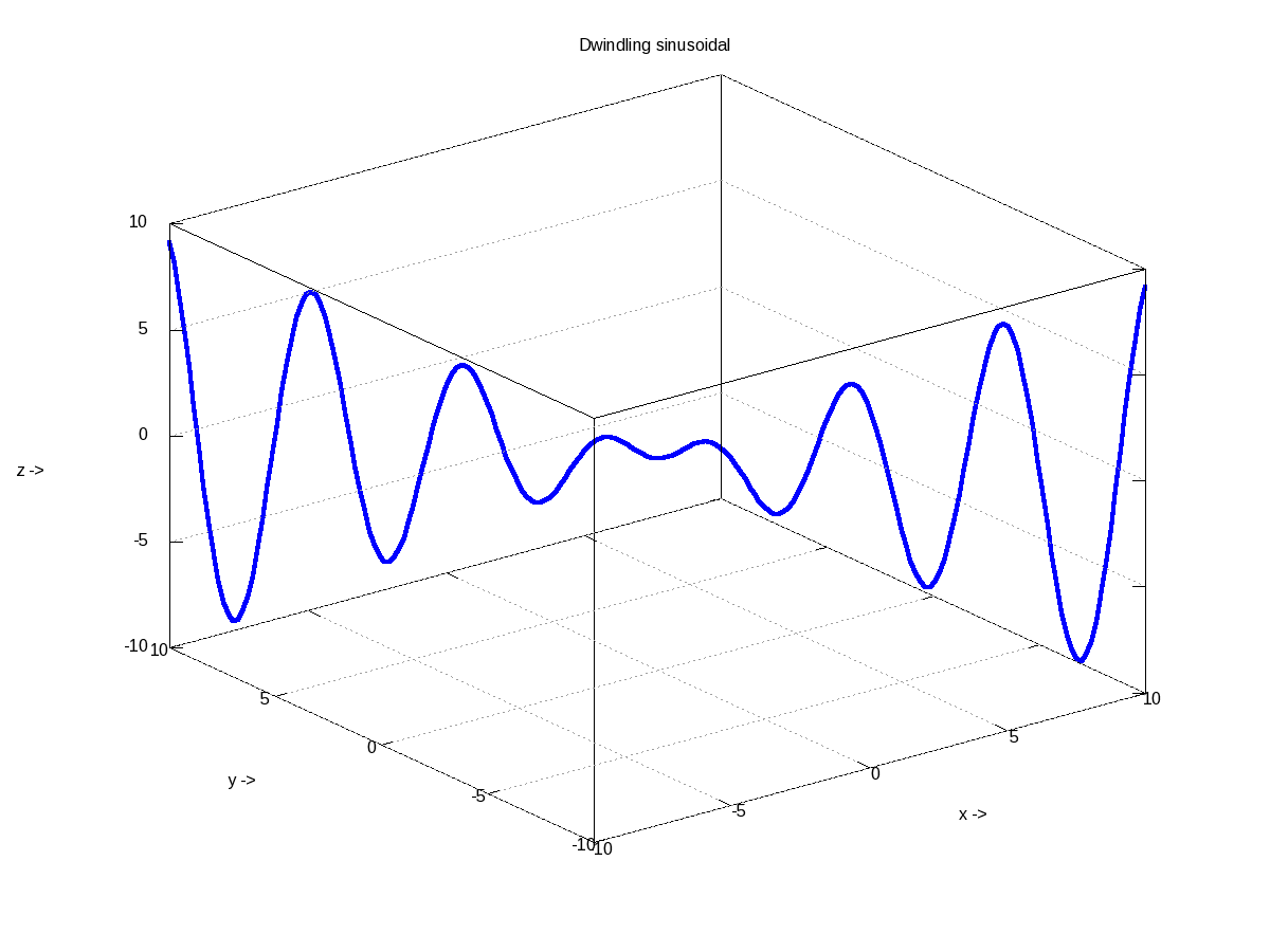
And finally, let’s do some 3-D plotting. plot3() is the simplest octave function to do a simple 3-D drawing, taking the set of (x, y, z) points. Here’s the sample code to draw the dwindling sinusoidal curve shown in Figure 17:

octave:1> x = -10:0.1:10;
octave:2> y = 10:-0.1:-10;
octave:3> z = x .* sin(x - y); 
octave:4> plot3(x, y, z, "-", "LineWidth", 4); 
octave:5> xlabel("x ->");
octave:6> ylabel("y ->");
octave:7> zlabel("z ->");
octave:8> title("Dwindling sinusoidal");
octave:9> grid("on");
octave:10>
Figure 17: 3-D plot of a dwindling sinusoidal

Figure 17: 3-D plot of a dwindling sinusoidal

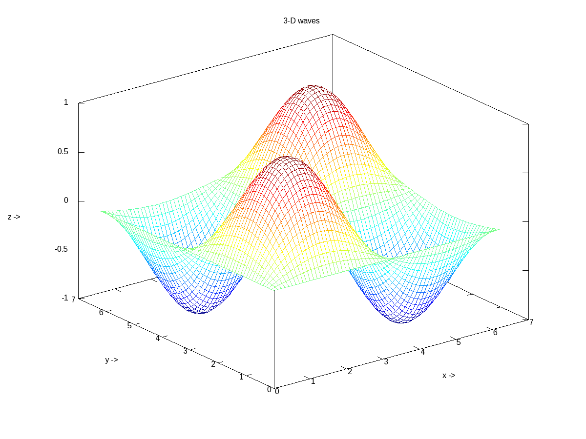
In case, we want to plot the values of a 2-D matrix against its indices (x, y), it could be done using mesh(), one of the many other 3-D plotting functions. Figure 18 shows the same, created using the following code:

octave:1> x = 0:0.1:2*pi;
octave:2> y = 0:0.1:2*pi;
octave:3> z = sin(x)' * sin(y);
octave:4> mesh(x, y, z); 
octave:5> xlabel("x ->");
octave:6> ylabel("y ->");
octave:7> zlabel("z ->");
octave:8> title("3-D waves");
octave:9>
Figure 18: 3-D waves

Figure 18: 3-D waves

What’s next?

Hope you enjoyed the colours of drawing. Next, we would look into octave from a statisticians perspective.

Thirteenth Article >>

   Send article as PDF   

Polynomial Curve Fitting & Interpolation

This eleventh article of the mathematical journey through open source, explains curve fitting & interpolation with polynomials in octave.

<< Tenth Article

In various fields of physics, chemistry, statistics, economics, … we very often come across something called curve fitting, and interpolation.

Given a set of data points from our observations, we would like to see what mathematical equation does they follow. So, we try to fit the best curve through those data points, called the curve fitting technique. Once we have the equation, the main advantage is that then we can find the values at the points, we haven’t observed by just substituting that value in the equation. One may think of this as interpolation. But this is not exactly interpolation. As in interpolation, we are restricted to finding unobserved values only between two observed points, using a pre-defined curve fit between those two points. With that we may not be able to get values outside our observation range. But the main reason for using that is when we are not interested or it is not meaningful or we are unable to fit a known form of curve in the overall data set, but still we want to get some approximations of values, in between the observed data points. Enough of gyaan, now let’s look into each one of those.

Curve Fitting

Let’s say for any system, we have the following data points:
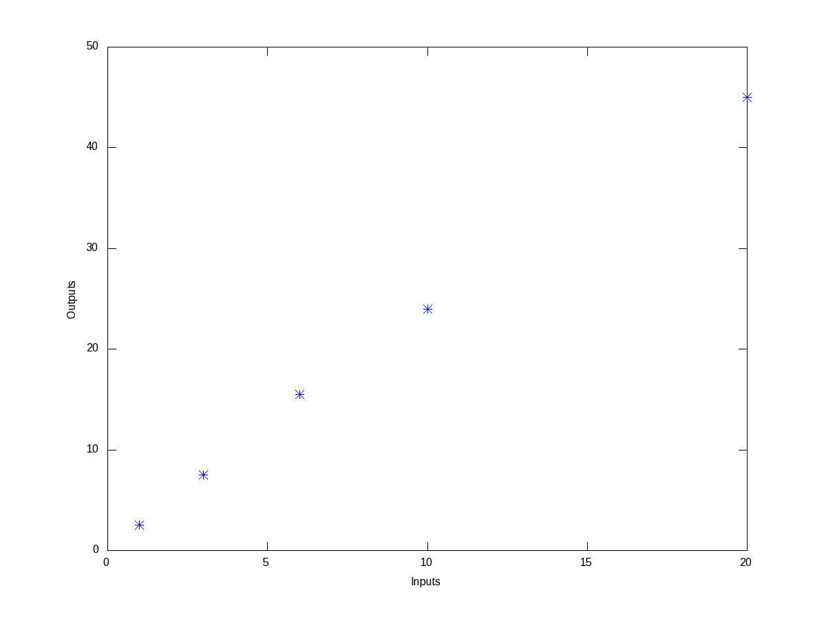
For the inputs of 1, 3, 6, 10, 20, we get the outputs as 2.5, 7.5, 15.5, 24, 45, respectively. Then, we would like to know as how is input is related to the output. So, to get a feel of the relation, we first plot this points on a x-y plane, say inputs as x and outputs as y. Figure 6 shows the same. And the octave code for that is as follows:

$ octave -qf
octave:1> x = [1 3 6 10 20];
octave:2> y = [2.5 7.5 15.5 24 45];
octave:3> plot(x, y, "*");
octave:4> xlabel("Inputs");
octave:5> ylabel("Outputs");
octave:6>
Figure 6: Plot of the data points

Figure 6: Plot of the data points

By observing the plot, the simplest fitting relation looks to be a straight line. So, let’s try fitting a linear polynomial, i.e. a first order polynomial, i.e. a straight line. Here’s the code in execution for it:

octave:1> x = [1 3 6 10 20];
octave:2> y = [2.5 7.5 15.5 24 45];
octave:3> p = polyfit(x, y, 1)
p =

   2.2212   1.1301

octave:4> polyout(p, "x");

2.2212*x^1 + 1.1301

octave:5> plot(x, y, "*", x, polyval(p, x), "-");
octave:6> xlabel("Inputs");
octave:7> ylabel("Outputs");
octave:8> legend("Data points", "Linear Fit");
octave:9>

polyfit() takes 3 arguments, the x values, the y values, and the order of the polynomial to fit – 1 for linear. It then returns the coefficients of the fitted polynomial p. polyout() displays the polynomial in more readable format. So, the fitted equation is y = 2.2212 * x + 1.1301. polyval() takes the polynomial p and the input values x, and calculates the output values y, as per the polynomial equation. And then we plot them, along with the earlier data points, on the same plot. Figure 7 shows the same, 2.2212 being the slope / gradient of the straight line, and 1.1301 being the intercept. Now, we notice that the straight line does not fit exactly, and there is some deviation from the observed points. polyfit() fits the polynomial with the minimum deviation for the order we request, but still there is a deviation, as that is the minimum possible. If you want to get the standard deviation for the particular fit, you just need to do the following:

octave:9> std_dev = sqrt(mean((y - polyval(p, x)).^2))
std_dev =  0.72637
octave:10>
Figure 7: Linear fit of data points

Figure 7: Linear fit of data points

And we see that it is a small value compared to our output values. But say we are not fully satisfied with this, we may like to try higher order polynomials, say of order 2, a quadratic, and observe the results from it. Here’s how one would do this:

octave:1> x = [1 3 6 10 20];
octave:2> y = [2.5 7.5 15.5 24 45];
octave:3> p = polyfit(x, y, 2)
p =

  -0.018639   2.623382  -0.051663

octave:4> polyout(p, "x");

-0.018639*x^2 + 2.6234*x^1 - 0.051663

octave:5> plot(x, y, "*", x, polyval(p, x), "-");
octave:6> xlabel("Inputs");
octave:7> ylabel("Outputs");
octave:8> legend("Data points", "Quadratic Fit");
octave:9> std_dev = sqrt(mean((y - polyval(p, x)).^2))
std_dev =  0.26873
octave:10>

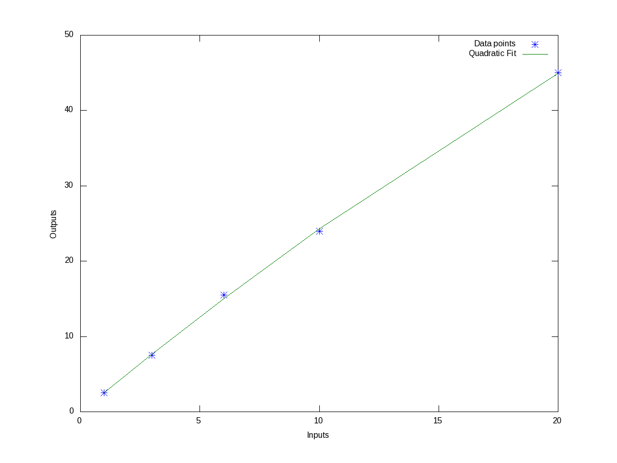
Figure 8 shows the data points and fitted quadratic curve. All the values above can be interpreted in the similar way as earlier. And we note that the standard deviation has come down further. In fact, as we increase the polynomial order further and further, we will definitely note that the standard deviation keeps on decreasing, till the order is same as number of data points – 1, after which it remains 0. But, we may not like to do this, as our observed data points are typically not perfect, and we are typically not interested in getting the standard deviation zero but for a fit more appropriate to reflect the relation between the system’s input and output.

Figure 8: Quadratic fit of data points

Figure 8: Quadratic fit of data points

Interpolation

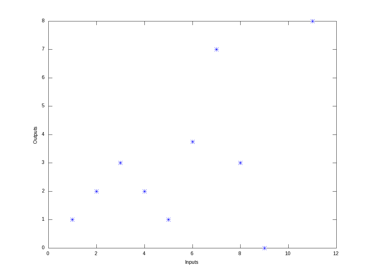
Now, say we have the following wierd data points, listed as (x, y) pairs: (1, 1), (2, 2), (3, 3), (4, 2), (5, 1), (6, 3.75), (7, 7), (8, 3), (9, 0), (11, 8). Figure 9 shows, how wierd they look like.

Figure 9: Wierd data points

Figure 9: Wierd data points

Trying to fit a polynomial, would be quite meaningless. But still they seem to have some correlation in between smaller ranges of input, say between 1 and 3, 3 and 5, 5 and 7, and so on. So, this is best suited for us to do interpolation for finding the values in between, say at 1.5, 3.8, 10, … Now interpolation is all about curve fitting between two neighbouring data points and then calculating the value at any intermediate point. So, the typical varieties of techniques used for this “piece-wise curve fitting” are:

  • nearest: Return the nearest data point (actually no curve fitting)
  • linear: Linear/Straight line fitting between the two neighbouring data points
  • pchip: Piece-wise cubic (order 3) hermite polynomial fitting
  • cubic: Cubic (order 3) polynomial fitted between four nearest neighbouring data points
  • spline: Cubic (order 3) spline fitting with smooth first and second derivatives throughout the curve

All these may look little jargonish – so don’t worry about that. Let’s just try out some examples to drive the point home. Here’s the code to show the nearest & linear interpolation for the above data:

octave:1> x = [1 2 3 4 5 6 7 8 9 11];
octave:2> y = [1 2 3 2 1 3.75 7 3 0 8];
octave:3> xi = 1:0.1:11;
octave:4> y_n = interp1(x, y, xi, "nearest");
octave:5> y_l = interp1(x, y, xi, "linear");
octave:6> plot(x, y, "*", xi, y_n, "-", xi, y_l, "-");
octave:7> xlabel("Inputs");
octave:8> ylabel("Outputs");
octave:9> legend("Data points", "Nearest", "Linear");
octave:10>

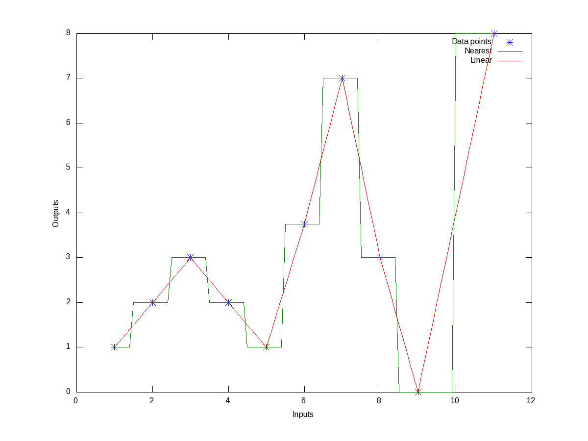
Figure 10 shows the same.

Figure 10: Nearest and linear interpolations of the data points

Figure 10: Nearest and linear interpolations of the data points

Now, if we want to get the interpolated values say at the points 1.5, 3.8, 10, instead of giving all the intermediate points xi in the above code, we may just give these 3 – that’s all. Here goes the code in execution for the that:

octave:1> x = [1 2 3 4 5 6 7 8 9 11];
octave:2> y = [1 2 3 2 1 3.75 7 3 0 8];
octave:3> our_x = [1.5 3.8 10];
octave:4> our_y_n = interp1(x, y, our_x, "nearest")
our_y_n =

   2   2   8

octave:5> our_y_l = interp1(x, y, our_x, "linear")
our_y_l =

   1.5000   2.2000   4.0000

octave:6>

Now, before closing on interpolation, just to give a feel of all of the interpolation techniques, here goes an example with the points on a sine curve:

octave:1> x = 0:2*pi;
octave:2> y = sin(x);
octave:3> xi = 0:0.1:2*pi;
octave:4> y_n = interp1(x, y, xi, "nearest");
octave:5> y_l = interp1(x, y, xi, "linear");
octave:6> y_p = interp1(x, y, xi, "pchip");
octave:7> y_c = interp1(x, y, xi, "cubic");
octave:8> y_s = interp1(x, y, xi, "spline");
octave:9> plot(x, y, "*", xi, y_n, "-", xi, y_l, "-", xi, y_p, "-", xi, y_c, "-",
                                                                      xi, y_s, "-");
octave:10> xlabel("x ->");
octave:11> ylabel("y ->");
octave:12> legend("Data points", "Nearest", "Linear", "Pchip", "Cubic", "Spline");
octave:13> print("-dpng", "all_types_of_interpolations.png");
octave:14>

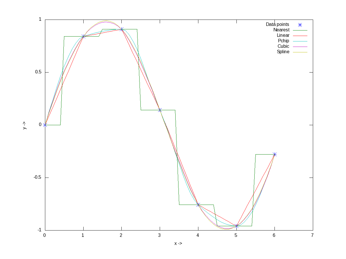
Figure 11 shows the visualization of the same for your eyes.

Figure 11: All types of interpolations for sinusoidal points

Figure 11: All types of interpolations for sinusoidal points

What’s next?

With today’s curve fitting & interpolation walk through, we have used some basic 2-D plotting techniques. But there are many more features and techniques to plotting, like marking our plots, visualizing 3-D stuff, etc. Next, we’ll look into that.

Twelfth Article >>

   Send article as PDF   

Polynomial Power of Octave

This tenth article of the mathematical journey through open source, explains advanced polynomial mathematics in octave.

<< Ninth Article

Roots of i

Let’s start with the solution to our previous brain teaser of finding the square and cube roots of the imaginary number i, which boils down to finding all the roots of the equations x2 = i and x3 = i, respectively. In other words, roots of the polynomials x2 – i and x3 – i, respectively, as follows:

$ octave -qf
octave:1> roots([1 0 -i])
ans =

   0.70711 + 0.70711i
  -0.70711 - 0.70711i

octave:2> roots([1 0 0 -i])
ans =

  -0.86603 + 0.50000i
  -0.00000 - 1.00000i
   0.86603 + 0.50000i

octave:3>

Displaying Polynomial

Before we start exploring polynomials further, here’s a couple of basic octave functions to visualize the polynomials. polyout() displays a polynomial in our usual known format. polyreduce() removes the redundant leading zero coefficients. Check out the following:

$ octave -qf
octave:1> p = [ 0 0 5 3 -9 4 6 ];
octave:2> polyout(p, "x");
0*x^6 + 0*x^5 + 5*x^4 + 3*x^3 - 9*x^2 + 4*x^1 + 6
octave:3> polyreduce(p)
ans =

   5   3  -9   4   6

octave:4> polyout(polyreduce(p), "x");
5*x^4 + 3*x^3 - 9*x^2 + 4*x^1 + 6
octave:5>

Polynomial Arithmetic

As octave represents polynomial as vectors, their addition and subtraction are vector addition and subtraction, respectively. However, the polynomial vectors may be of different length. Hence, they need to be made of same length before addition or subtraction. So, let’s write functions to do the complete operations:

function [ q1 q2 ] = equalize(p1, p2)
# Assuming p1 & p2 to be row vectors
    m = max(length(p1), length(p2));
    q1 = [ zeros(1, m - length(p1)) p1 ];
    q2 = [ zeros(1, m - length(p2)) p2 ];
endfunction

function p = polyadd(p1, p2)
    [ q1 q2 ] = equalize(p1, p2);
    p = polyreduce(q1 + q2);
endfunction

function p = polysub(p1, p2)
    [ q1 q2 ] = equalize(p1, p2);
    p = polyreduce(q1 - q2);
endfunction

Assuming the above code is put in the file polynomials.oct, the same can be used as follows:

$ octave -qf
octave:1> source("polynomials.oct");
octave:2> polyout(p1 = [ 1 2 1 ], "x");
1*x^2 + 2*x^1 + 1
octave:3> polyout(p2 = [ 1 -1 ], "x");
1*x^1 - 1
octave:4> polyout(polyadd(p1, p2), "x");
1*x^2 + 3*x^1 + 0
octave:5> polyout(polysub(p1, p2), "x");
1*x^2 + 1*x^1 + 2
octave:6>

Interestingly, octave already have the functions for multiplication and division of polynomials, namely conv() and deconv(), respectively. Here’s a demonstration:

$ octave -qf
octave:1> polyout(p1 = [ 1 2 1 ], "x");
1*x^2 + 2*x^1 + 1
octave:2> polyout(p2 = [ 1 -1 ], "x");
1*x^1 - 1
octave:3> polyout(conv(p1, p2), "x");
1*x^3 + 1*x^2 - 1*x^1 - 1
octave:4> polyout(deconv(p1, p2), "x");
1*x^1 + 3
octave:5> [ q r ] = deconv(p1, p2)
q =

   1   3

r =

   0   0   4

octave:6>

Polynomial Differentiation and Integration

Octave also provides functions for differentiation and integration of polynomials, namely polyder() and polyint(). Here goes an example of differentiation and definite integral using the same:

$ octave -qf
octave:1> polyout(p = [ 1 2 1 ], "x");
1*x^2 + 2*x^1 + 1
octave:2> polyout(polyder(p), "x");
2*x^1 + 2
octave:3> polyout(polyint(p), "x");
0.33333*x^3 + 1*x^2 + 1*x^1 + 0
octave:4> q = polyint(p);
octave:5> polyval(q, 3) - polyval(q, 0) # Definite integral of p from 0 to 3
ans =  21
octave:6>

What’s next?

Given a set of data points a common requirement in fields of physics, statistics, and many others is to fit a polynomial to it. Going further, we’ll explore the power of octave for the same.

Eleventh Article >>

   Send article as PDF   

Get Set with Polynomials in Octave

This ninth article of the mathematical journey through open source, deals with polynomial mathematics in octave.

<< Eighth Article

Let’s first solve the earlier puzzles. And then we shall discuss the polynomial power of octave.

Number Puzzle

Find three numbers, product of which is 60; sum of their squares is 50; and their sum is 12. Let the X vector elements X(1), X(2), X(3) be the three numbers. Then, here goes the solution:

$ octave -qf
octave:1> function Y = F(X)
> Y(1) = X(1) * X(2) * X(3) - 60; 
> Y(2) = X(1)^2 + X(2)^2 + X(3)^2 - 50; 
> Y(3) = X(1) + X(2) + X(3) - 12; 
> endfunction
octave:2> [Y, Fval, info] = fsolve(@F, [3; 3; 3]) 
warning: matrix singular to machine precision, rcond = 4.32582e-35
warning: attempting to find minimum norm solution
warning: dgelsd: rank deficient 3x3 matrix, rank = 1 
Y =

   5.0000
   3.0000
   4.0000

Fval =

  -3.2345e-07   1.0351e-07   0.0000e+00

info = 1 
octave:3>

So, the 3 numbers are 5, 3, 4.

Flower Puzzle

A sage came to a temple with some flowers and dipped them into the first pond of the temple to get them squared. Then, he offered some flowers in the temple and dipped the remaining flowers into the second pond to get them doubled. Then, he again offered same number of flowers, as earlier, and dipped the remaining flowers into the third pond to get them tripled and take back with him as prasadam, which was the same number as in each one of his offerings. Now, if he took back thrice the number of flowers he brought. How many did he bring in with him?
Let the x vector elements x(1) and x(2) be respectively, the number of flowers the sage came with and the number of flowers the sage offered each time. So, here goes the solution:

octave:1> function y = f(x)
> y(1) = ((x(1) * x(1) - x(2)) * 2 - x(2)) * 3 - x(2);
> y(2) = x(2) - 3 * x(1);
> endfunction 
octave:2> [x fval info] = fsolve(@f, [10; 10])
x =

    5.0000
   15.0000

fval =

  -2.8791e-06  -1.7764e-15

info =  1
octave:3>

So, the number of flowers the sage came with is 5 and his each offering is of 15 flowers.

Note that in all these solutions the trick is to choose the initial solution close to the original solution, through some approximation work. At times that might be tricky. So, in case we just have polynomial equations and that also in one variable, it can be solved in an easier way, using the polynomial features of octave. In contrast to the earlier method, here we also get all of the multiple solutions for the polynomial.

Playing with Polynomials

Let’s consider the polynomial equation 2x3 + 3x2 + 2x + 1 = 0. Then its octave representation and computation of its solutions aka roots would be as follows:

octave:1> P = [2; 3; 2; 1];
octave:2> roots(P)
ans =

  -1.00000 + 0.00000i
  -0.25000 + 0.66144i
  -0.25000 - 0.66144i

octave:3>

So, it being a cubic equation, it has three roots as expected. First one is the real number -1, and the other two are complex conjugates (-1 + sqrt(-7))/4 & (-1 – sqrt(-7))/4. And you may verify the solutions using the function polyval() as follows:

octave:1> P = [2; 3; 2; 1];
octave:2> sols = [-1; (-1 + sqrt(-7)) / 4; (-1 + sqrt(-7)) / 4]
sols =

  -1.00000 + 0.00000i
  -0.25000 + 0.66144i
  -0.25000 + 0.66144i

octave:3> polyval(P, sols)
ans =

   0
   0
   0

octave:4>

This shows that the value of the polynomial P evaluated at each of the 3 solutions is 0. Hence, confirming that they indeed are the solutions.

All set with polynomial basics in octave, let’s solve some puzzles.

Geometry Solving

Last time we found an intersection point of a straight line and a circle. Yes, we just calculated one point – though typically there would be two. It would be one only in case of the straight line being tangent or just touching the circle. And yes it would be zero, if the straight line is not even intersecting it. So now, let’s try these different cases, with the one variable polynomial power.

Let us have the following circle C with radius 5 and centered at origin (0, 0), defined in the Cartesian coordinate system, i.e. the x-y system: x2 + y2 = 25

And, let us consider the following 3 lines for intersection with the above circle, one by one:

  • L1: 4x + 3y = 24
  • L2: x + y = 5√2
  • L3: 6x + y = 36

To be able to solve for the intersection points of each of these 3 lines with the circle C using roots, the first step is to get polynomials in one variable. For that, we can substitute the value of y in the equation of the circle, in terms of x from each of the line equations, as follows:
For L1
x2 + y2 = 25 ⇒ 9x2 + 9y2 = 9*25 ⇒ 9x2 + (24 – 4x)2 = 225 ⇒ 25x2 – 192x + 351 = 0
For L2
x2 + y2 = 25 ⇒ x2 + (5√2 – x)2 = 25 ⇒ 2x2 – 10√2x + 25 = 0
For L3
x2 + y2 = 25 ⇒ x2 + (36 – 6x)2 = 25 ⇒ 37x2 – 432x + 1271 = 0

Now, we get the roots of each to get the x co-ordinate of the intersection point.

octave:1> C1 = [25; -192; 351];
octave:2> C2 = [2; -10*sqrt(2); 25];
octave:3> C3 = [37; -432; 1271];
octave:4> roots(C1)
ans =

   4.6800
   3.0000

octave:5> roots(C2)
ans =

   3.5355
   3.5355

octave:6> roots(C3)
ans =

   5.8378 + 0.5206i
   5.8378 - 0.5206i

octave:7>

And the corresponding y co-ordinate could be obtained by substituting the value of x into the corresponding line equations.

For L1, there are 2 different roots 4.68 and 3, implying two intersecting points (4.68, 1.76) and (3, 4).
For L2, there are 2 identical roots of 3.5355 i.e 5/√2, implying just one intersecting point (5/√2, 5/√2).
For L3, the roots are complex, implying that there is no intersecting point in the real world.

Solve it

And finally, here’s one for your brain. Find out the two square roots and the three cube roots of the imaginary number i.

If you think, you have got the octave code for solving the above, post your solution in the comments below. And as we move on, we would have more fun with the polynomials.

Tenth Article >>

   Send article as PDF   

Solve Non-linear Equations using Linear Algebra

This eighth article of the mathematical journey through open source, solves non-linear equations using linear algebra in octave.

<< Seventh Article

Hope you have found out the vegetable prices from the vegetable seller, who had placed various equal priced stacks for sell at ₹30. Recall: One stack had 4 lemons, 7 cucumbers, 9 tomatoes. Another had 2 lemons, 5 cucumbers, 27 tomatoes. And the third had just 9 cucumbers & 15 tomatoes. Prices would be ₹2.00 per lemon, ₹2.50 per cucumber, ₹0.50 per tomato, computed as follows:

$ octave -qf
octave:1> N = [
> 4 7 9
> 2 5 27
> 0 9 15
> ];
octave:2> inv(N) * [30; 30; 30]
ans =

   2.00000
   2.50000
   0.50000

octave:3>

Polynomial solving

Note that though in 3 variables, even this was a linear equation. How about solving higher order polynomial equations, meaning of squares, cubes, … of the variables. Say, we want a solution for x in x3 + 3x2 + 3x + 1 = 0. Simple! First define a function for this polynomial. And, then use the function solver fsolve() to solve it, as follows:

$ octave -qf
octave:1> function y = f(x)
> y = x^3 + 3*x^2 + 3*x + 1;
> endfunction
octave:2> [x, fval, info] = fsolve(@f, 0)
x = -0.99999
fval = 0
info =  1
octave:3>

This indicates the value of x as -0.99999 ≈ -1 as the solution to the function f(x), yielding a function value of 0, with info = 1 indicating that solution is obtained. And you may verify the answer by calling the function f with the variable x as f(x) on the octave prompt. The second parameter in fsolve() is the initial guess of the solution.

Geometry solving

With the power in hand, why not solve more complex geometric problems? Last time we found the intersection point of two straight lines. How about intersection of a straight line and a circle? Let us have the following straight line and circle, defined in the Cartesian coordinate system, i.e. the x-y system:
4x + 3y = 24
x2 + y2 = 25

To be able to solve it using fsolve(), let’s consider the different variables x & y as fields of a vector X, say x as X(1), y as X(2). Then, the equations can be re-written as follows:
4 * X(1) + 3 * X(2) = 24
X(1)^2 + X(2)^2 = 25
and hence could be solved using fsolve() as follows:

$ octave -qf
octave:1> function Y = F(X)
> Y(1) = 4 * X(1) + 3 * X(2) - 24;
> Y(2) = X(1)^2 + X(2)^2 - 25;
> endfunction
octave:2> [Y, Fval, info] = fsolve(@F, [0; 0])
warning: matrix singular to machine precision, rcond = 0
warning: attempting to find minimum norm solution
warning: dgelsd: rank deficient 2x2 matrix, rank = 1
Y =

   3.0000
   4.0000

Fval =

   0.0000e+00   2.6691e-07

info =  1
octave:3>

So, (3, 4) is the intersecting point – can be verified by substituting back into the above equations.

Solve it

Equipped with this knowledge, here’s a couple of teasers for your brain:

  1. Find three numbers, product of which is 60; sum of their squares is 50; and their sum is 12.
  2. A sage came to a temple with some flowers and dipped all of them into the first magical pond of the temple and got those back, squared. Then, he offered some of those flowers in the temple and dipped the remaining flowers into the second magical pond to get those back, doubled. Then, he again offered the same number of flowers, as offered earlier, and dipped the remaining flowers into the third magical pond to get those back, tripled, which he took back with him as prasadam. Now, the number of flowers he took back with him, is same as in each one of his offerings. Also, what he took back with him is thrice the number of flowers he came with to the temple. How many flowers did he come in with?

If you think, you have got the octave code for solving the above, you may post the solution in the comments below. And as we move on, we would get into specifically playing with polynomials.

Ninth Article >>

   Send article as PDF   

Solve Puzzles using Linear Algebra

This seventh article of the mathematical journey through open source, solves puzzles using linear algebra in octave.

<< Sixth Article

Matrix Maths is what is formally called Linear Algebra. We have gone through its basics in the fifth article. Now, we shall apply that to practical usage. What better than solving puzzles using the same.

Purchase Solving

Shrishti purchased 24 pencils and 12 erasers for ₹96. Divya purchased 20 pencils and 15 erasers for ₹100. What are the prices of the pencil & the eraser?

Assuming that ‘p’ is the price for pencils & ‘e’ is the price for erasers, we have the following two equations:
24 * p + 12 * e = 96
20 * p + 15 * e = 100
Hence, we could get the values of ‘p’ & ‘e’ by solving these equations. Converting them into linear algebra form, they can be re-written using matrix multiplication as:
┏          ┓┏    ┓    ┏        ┓
┃24 12 ┃┃ p ┃    ┃   96 ┃
┃20 15 ┃┃ e ┃ = ┃ 100 ┃
┗          ┛┗    ┛    ┗        ┛
which is Ax = b, ‘x’ being the vector with variables ‘p’ & ‘e’. Hence, we need to solve for x, which is given by: x = A-1b. Using octave:

$ octave -qf
octave:1> A = [
> 24 12
> 20 15
> ];
octave:2> b = [
> 96
> 100
> ];
octave:3> x = inv(A) * b
x =

   2.0000
   4.0000

octave:4>

Hence, p = ₹2 and e = ₹4, i.e. each pencil costs ₹2 and an eraser costs ₹4. You may check by putting back these values in our problem statement. Isn’t that cool?

Geometry Solving

How about finding the intersection point of two straight lines? Let us have the following 2 straight lines, defined in the Cartesian coordinate system, i.e. the x-y system:
4x + 3y = 24
3x + 4y = 25

Similar to the earlier problem, the intersecting point could be obtained as follows:

$ octave -qf
octave:1> A = [
> 4 3
> 3 4
> ];
octave:2> b = [
> 24
> 25
> ];
octave:3> X = inv(A) * b
X =

   3.0000
   4.0000

octave:4>

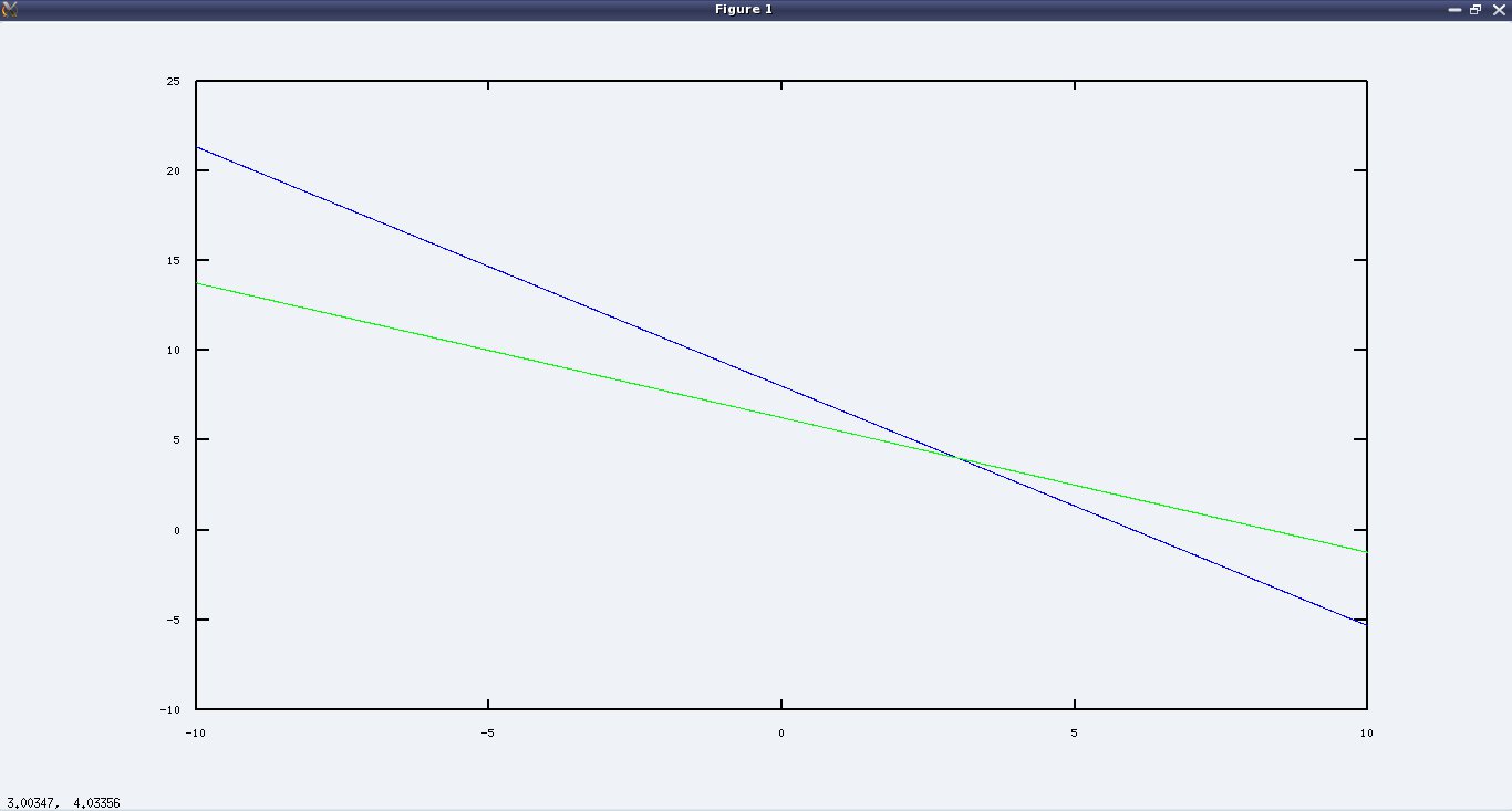
So, (3, 4) is the intersecting point. Want to see it visually. For that, we would just need to rewrite the straight line equations as follows:
y = (24 – 4x) / 3
y = (25 – 3x) / 4
And then here goes the code:

octave:1> x=-10:0.01:10;
octave:2> plot(x, (24 - 4*x)/3, "b.", x, (25 - 3*x)/4, "g.");
octave:3>

Figure 5 shows the plot generated by the above code.

Figure 5: Intersection of straight lines

Figure 5: Intersection of straight lines

Solve it

Equipped with the puzzle solving basics, here’s one for your brain: A vegetable seller has placed various equal priced stacks for sale at ₹30. One stack has 4 lemons, 7 cucumbers, 9 tomatoes. Another has 2 lemons, 5 cucumbers, 27 tomatoes. And the third has just 9 cucumbers & 15 tomatoes. Can you compute the price of each vegetable?

Hint: Assume the price of lemon, cucumber, tomato as ‘l’, ‘c’, ‘t’, and then form the 3 equations in three variables.

If you think, you have got it, you may post the solution in the comments. And as we move on, we will get into some different kind of puzzle solving.

Eighth Article >>

   Send article as PDF   

The Imaginary Music of Octave

This sixth article of the mathematical journey through open source, introduces you to the imaginary numbers through octave.

<< Fifth Article

Yes, we have done the powerful matrix math with octave, without even thinking of how it is internally done. Now, on the same note, let’s continue to explore one of the most fascinating or rather most imaginary stuff of math.

i Fun

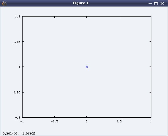
Yes what else the imaginary numbers, numbers which really don’t exist but we try to visualize them as points on a 2-D plane with the real part on x-axis and the imaginary part on y-axis. So to plot the imaginary i, with a blue star (*), issue the following command at the octave prompt:

$ octave -qf
octave:1> plot(i, "b*")
octave:2>

and here pops the display window as shown in Figure 3.

Figure 3: Plot of i (sqrt(-1))

Figure 3: Plot of i (sqrt(-1))

What is this i? Just square root of -1. Simple! Right? Remember, we got an error trying sqrt(-1) in bc. octave is neat. It will answer you politely with an i. Still confused. Just check out the following:

$ octave -qf
octave:1> i
ans =  0 + 1i
octave:2> i * i
ans = -1
octave:3> sqrt(-1)
ans =  0 + 1i
octave:4> i^3
ans = -0 - 1i
octave:5>

i Puzzle

And now comes the puzzle part. What is the imaginary part of ii? It’s zero. What? Is it a real number? Yes it is. It is in fact equal to e-π/2. Check out for yourself:

$ octave -qf
octave:1> i^i
ans =  0.20788
octave:2> exp(-pi/2)
ans =  0.20788
octave:3> 

Yes, you don’t really need to bother about how. octave just gets you there. And that’s fun with mathematics without getting into mathematics.

i: just a number

If you are not puzzled by this, great! In fact, as the imaginary numbers are numbers, just special numbers, in octave, they can be used in any operations you may think of with numbers. Try out sqrt, exp, log – addition, subtraction, multiplication, division are just trivial ones. And more fun would be with the octave power of vectors & matrices. Watch out:

$ octave -qf
octave:1> sqrt(i)
ans =  0.70711 + 0.70711i
octave:2> exp(i)
ans =  0.54030 + 0.84147i
octave:3> log(i)
ans =  0.00000 + 1.57080i
octave:4>  [i  # Press <Enter> here
>           i] * [i i]
ans =

  -1  -1
  -1  -1

octave:5>

Is e really cos θ + i sin θ?

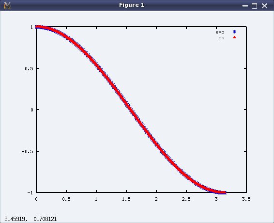
A very simple check. Let’s plot both the curves. Let θ (theta) be set to values from 0 to π (pi) with say intervals of 0.01, and then let’s plot the two curves in blue and red:

$ octave -qf
octave:1> th=0:0.01:pi;
octave:2> plot(th, exp(i*th), "b*;exp;", th, cos(th)+i*sin(th), "r^;cs;")
octave:3> 

Figure 4 shows the plot with the 2 curves coinciding exactly with each other.

Figure 4: Plot of Euler's equality

Figure 4: Plot of Euler’s equality

Equipped with i, let’s play out with more puzzles, as we move on. Get ready with octave controls.

Seventh Article >>

   Send article as PDF   

Mathematics made easy with minimal Octave

This fifth article of the mathematical journey through open source, introduces the minimal, octave can do for you.

<< Fourth Article

You wanted a non-programmers way of doing mathematics and there you go – octave. Sounds like something to do with music, but in reality it is the name the octave author’s chemical engineering professor, who was well know for his ‘back of the envelope’ calculations.

All of bench calculator!!!

All the operations of bench calculator are just a subset of octave. So, no point going round the wheel again. Whatever operations can be done in bc – arithmetic, logical, relational, conditional – all can be done with equal ease in octave. As in bc, it can as well be used as a mathematical programming language. Ha! Then, why did we waste time on learning bc, we could have straight away come to octave. Yes! Yes! Except one thing – the precision-less-ness. We can’t get that in octave. If we need that, we would have to go back to bc. Okay! Fine. So, what with octave – we start with N-dimensions, what else. Hey don’t worry! In simple language, I mean vectors & matrices.

Getting Started

Command: Typing ‘octave‘ on the shell brings up the octave‘s interactive shell. Type ‘quit’ or Control-D to exit. The interactive shell starts with a welcome message. As in bc, we pass option -q for it to not show. Additionally, we’ll use the -f option for it to not pick any local start-up scripts (if any). So, for our examples, the command would look like ‘octave -qf‘ to start octave with an interactive shell.

Prompts & Results: Input prompt is typically denoted by ‘octave:X>‘, where X just a number showing the command count. Valid results are typically shown with ‘<variable> = ‘, or ‘ans = ‘ or ‘=> ‘, and then the command count incremented for the next input. Errors cause error messages to be printed and then octave brings back the input prompt without incrementing the command count. Putting a semicolon (;) at the end of an statement, suppresses it result (return value) to be displayed.

Comments could start with # or %. For block comments, #{ … }# or %{ … }% can be used.

Detailed topic help could be obtained using ‘help <topic>’ or complete documentation using ‘doc’ on the octave shell.

All in a go:

$ octave -qf
octave:1> # This is a comment
octave:1> pi # Built-in constant
ans =  3.1416
octave:2> e # Built-in constant again
ans =  2.7183
octave:3> i # Same as j – the imaginary number
ans =  0 + 1i
octave:4> x = 3^4 + 2*30;
octave:5> x
x =  141
octave:6> y
error: `y' undefined near line 6 column 1
octave:6> doc # Complete doc; Press 'q' to come back
octave:7> help plot # Help on plot
octave:8> A = [1 2 3; 4 5 6; 7 8 9] # 3x3 matrix
A =

   1   2   3
   4   5   6
   7   8   9

octave:9> quit

Matrices with a Heart

Yes, we already saw a matrix in creation. It can also be created through multiple lines. Octave continues waiting for further input by prompting just ‘>’. Checkout below for creating the 3×3 magic square matrix in the same way, followed by various other interesting operations:

$ octave -qf
octave:1> M = [ # 3x3 magic square
> 8 1 6
> 3 5 7
> 4 9 2
> ]
M =

   8   1   6
   3   5   7
   4   9   2

octave:2> B = rand(3, 4); # 3x4 matrix w/ randoms in [0 1]
octave:3> B
B =

   0.068885   0.885998   0.542059   0.797678
   0.652617   0.904360   0.036035   0.737404
   0.043852   0.579838   0.709194   0.053118

octave:4> B' # Transpose of B
ans =

   0.068885   0.652617   0.043852
   0.885998   0.904360   0.579838
   0.542059   0.036035   0.709194
   0.797678   0.737404   0.053118

octave:5> A = inv(M) # Inverse of M
A =

   0.147222  -0.144444   0.063889
  -0.061111   0.022222   0.105556
  -0.019444   0.188889  -0.102778

octave:6> M * A # Should be identity, at least approx.
ans =

   1.00000   0.00000  -0.00000
  -0.00000   1.00000   0.00000
   0.00000   0.00000   1.00000

octave:7> function rv = psine(x) # Our phase shifted sine
>
> rv = sin(x + pi / 6);
>
>  endfunction 
octave:8> x = linspace(0, 2*pi, 400); # 400 pts from 0 to 2*pi
octave:9> plot(x, psine(x)) # Our function's plot
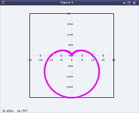
octave:10> polar(x, 10 * (1 - sin(x)), 'm*') # bonus Heart
octave:11> quit

Figure 1 shows the plot window which pops up by the command # 9 – plot.

Figure 2 is the bonus magenta heart of stars (*) from polar coordinates draw command # 10 – polar.

Figure 1: Plot of our 30° phase shifted sine

Figure 1: Plot of our 30° phase shifted sine

Figure 2: The Heart

Figure 2: The Heart

What next?

With ready-to-go level of introduction to octave, we are all set to explore it the fun way. What fun? Next one left to your imagination. And as we move on, we would take up one or more fun challenge(s), and try to see, how we solve it using octave.

Sixth Article >>

   Send article as PDF